A Method for Stopping Active Learning Based on Stabilizing Predictions and the Need for User Adjustable Stopping

A Method for Stopping Active Learning Based on Stabilizing Predictions

and the Need for User-Adjustable Stopping

Michael Bloodgood∗ Human Language Technology

Center of Excellence Johns Hopkins University Baltimore, MD 21211 USA

bloodgood@jhu.edu

K. Vijay-Shanker Computer and Information

Sciences Department University of Delaware Newark, DE 19716 USA vijay@cis.udel.edu

Abstract

A survey of existing methods for stopping ac-tive learning (AL) reveals the needs for meth-ods that are: more widely applicable; more ag-gressive in saving annotations; and more sta-ble across changing datasets. A new method for stopping AL based on stabilizing predic-tions is presented that addresses these needs. Furthermore, stopping methods are required to handle a broad range of different annota-tion/performance tradeoff valuations. Despite this, the existing body of work is dominated by conservative methods with little (if any) at-tention paid to providing users with control over the behavior of stopping methods. The proposed method is shown to fill a gap in the level of aggressiveness available for stopping AL and supports providing users with control over stopping behavior.

1 Introduction

The use of Active Learning (AL) to reduce NLP an-notation costs has generated considerable interest re-cently (e.g. (Bloodgood and Vijay-Shanker, 2009; Baldridge and Osborne, 2008; Zhu et al., 2008a)). To realize the savings in annotation efforts that AL enables, we must have a mechanism for knowing when to stop the annotation process.

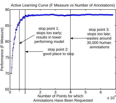
Figure 1 is intended to motivate the value of stop-ping at the right time. The x-axis measures the num-ber of human annotations that have been requested and ranges from 0 to 70,000. The y-axis measures

∗_{This research was conducted while the first author was a} PhD student at the University of Delaware.

0 1 2 3 4 5 6 7

x 104 65

70 75 80 85 90

Active Learning Curve (F Measure vs Number of Annotations)

Number of Points for which Annotations Have Been Requested

Performance (F Measure)

stop point 1: stops too early; results in lower performing model

stop point 2: good place to stop

stop point 3: stops too late; wastes around 30,000 human annotations

Figure 1: Hypothetical Active Learning Curve with hy-pothetical stopping points.

performance in terms of F-Measure. As can be seen from the figure, the issue is that if we stop too early while useful generalizations are still being made, we wind up with a lower performing system but if we stop too late after all the useful generalizations have been made, we just wind up wasting human annota-tion effort.

The terms aggressive and conservative will be used throughout the rest of this paper to describe the behavior of stopping methods. Conservative meth-ods tend to stop further to the right in Figure 1. They are conservative in the sense that they’re very careful not to risk losing significant amounts of F-measure, even if it means annotating many more ex-amples than necessary. Aggressive methods, on the other hand, tend to stop further to the left in Figure 1. They are aggressively trying to reduce unnecessary annotations.

There has been a flurry of recent work tackling the

problem of automatically determining when to stop AL (see Section 2). There are three areas where this body of work can be improved:

applicability Several of the leading methods are

re-stricted to only being used in certain situations, e.g., they can’t be used with some base learn-ers, they have to select points in certain batch sizes during AL, etc. (See Section 2 for dis-cussion of the exact applicability constraints of existing methods.)

lack of aggressive stopping The leading methods

tend to find stop points that are too far to the right in Figure 1. (See Section 4 for empirical confirmation of this.)

instability Some of the leading methods work well

on some datasets but then can completely break down on other datasets, either stopping way too late and wasting enormous amounts of annota-tion effort or stopping way too early and losing large amounts of F-measure. (See Section 4 for empirical confirmation of this.)

This paper presents a new stopping method based on stabilizing predictions that addresses each of these areas and provides user-adjustable stopping behavior. The essential idea behind the new method is to test the predictions of the recently learned mod-els (during AL) on examples which don’t have to be labeled and stop when the predictions have sta-bilized. Some of the main advantages of the new method are that: it requires no additional labeled data, it’s widely applicable, it fills a need for a method which can aggressively save annotations, it has stable performance, and it provides users with control over how aggressively/conservatively to stop AL.

Section 2 discusses related work. Section 3 ex-plains our Stabilizing Predictions (SP) stopping cri-terion in detail. Section 4 evaluates the SP method and discusses results. Section 5 concludes.

2 Related Work

Laws and Sch¨utze (2008) present stopping criteria based on the gradient of performance estimates and the gradient of confidence estimates. Their tech-nique with gradient of performance estimates is only

applicable when probabilistic base learners are used. The gradient of confidence estimates method is more generally applicable (e.g., it can be applied with our experiments where we use SVMs as the base learner). This method, denoted by LS2008 in Tables and Figures, measures the rate of change of model confidence over a window of recent points and when the gradient falls below a threshold, AL is stopped.

The margin exhaustion stopping criterion was de-veloped for AL with SVMs (AL-SVM). It says to stop when all of the remaining unlabeled examples are outside of the current model’s margin (Schohn and Cohn, 2000) and is denoted as SC2000 in Ta-bles and Figures. Ertekin et al. (2007) developed a similar technique that stops when the number of sup-port vectors saturates. This is equivalent to margin exhaustion in all of our experiments so this method is not shown explicitly in Tables and Figures. Since we use AL with SVMs, we will compare with mar-gin exhaustion in our evaluation section. Unlike our SP method, margin exhaustion is only applicable for use with margin-based methods such as SVMs and can’t be used with other base learners such as Maxi-mum Entropy, Naive Bayes, and others. Schohn and Cohn (2000) show in their experiments that margin exhaustion has a tendency to stop late. This is fur-ther confirmed in our experiments in Section 4.

The confidence-based stopping criterion (here-after, V2008) in (Vlachos, 2008) says to stop when model confidence consistently drops. As pointed out by (Vlachos, 2008), this stopping criterion is based on the assumption that the learner/feature represen-tation is incapable of fully explaining all the exam-ples. However, this assumption is often violated and then the performance of the method suffers (see Sec-tion 4).

thresh-old for min-err. They refuse to stop and they raise the min-err threshold if there have been any classi-fication changes on the remaining unlabeled data by consecutive actively learned models when the cur-rent min-err threshold is satisfied. We denote this multi-criteria-based strategy, reported to work better than min-err in isolation, by ZWH2008. As seen in (Zhu et al., 2008a), sometimes min-err indeed stops later than desired and ZWH2008 must (by nature of how it operates) stop at least as late as min-err does. The susceptibility of ZWH2008 to stopping late is further shown emprically in Section 4. Also, ZWH2008 is not applicable for use with AL setups that select examples in small batches.

3 A Method for Stopping Active Learning Based on Stabilizing Predictions

To stop active learning at the point when annotations stop providing increases in performance, perhaps the most straightforward way is to use a separate set of labeled data and stop when performance begins to level off on that set. But the problem with this is that it requires additional labeled data which is counter to our original reason for using AL in the first place. Our hypothesis is that we can sense when to stop AL by looking at (only) the predictions of consecutively learned models on examples that don’t have to be labeled. We won’t know if the predictions are cor-rect or not but we can see if they have stabilized. If the predictions have stabilized, we hypothesize that the performance of the models will have stabilized

and vice-versa, which will ensure a (much-needed)

aggressive approach to saving annotations.

SP checks for stabilization of predictions on a set of examples, called the stop set, that don’t have to be labeled. Since stabilizing predictions on the stop set is going to be used as an indication that model stabilization has occurred, the stop set ought to be representative of the types of examples that will be encountered at application time. There are two con-flicting factors in deciding upon the size of the stop set to use. On the one hand, a small set is desir-able because then SP can be checked quickly. On the other hand, a large set is desired to ensure we don’t make a decision based on a set that isn’t repre-sentative of the application space. As a compromise between these factors, we chose a size of 2000. In

Section 4, sensitivity analysis to stop set size is per-formed and more principled methods for determin-ing stop set size and makeup are discussed.

It’s important to allow the examples in the stop set to be queried if the active learner selects them because they may be highly informative and ruling them out could hurt performance. In preliminary ex-periments we had made the stop set distinct from the set of unlabeled points made available for querying and we saw performance was qualitatively the same but the AL curve was translated down by a few F-measure points. Therefore, we allow the points in the stop set to be selected during AL.1

The essential idea is to compare successive mod-els’ predictions on the stop set to see if they have stabilized. A simple way to define agreement be-tween two models would be to measure the percent-age of points on which the models make the same predictions. However, experimental results on a sep-arate development dataset show then that the cutoff agreement at which to stop is sensitive to the dataset being used. This is because different datasets have different levels of agreement that can be expected by chance and simple percent agreement doesn’t adjust for this.

Measurement of agreement between human anno-tators has received significant attention and in that context, the drawbacks of using percent agreement have been recognized (Artstein and Poesio, 2008). Alternative metrics have been proposed that take chance agreement into account. In (Artstein and Poesio, 2008), a survey of several agreement met-rics is presented. Most of the agreement metmet-rics are of the form:

agreement= Ao−Ae

1₋Ae

, (1)

whereAo =observed agreement, and Ae = agree-ment expected by chance. The different metrics dif-fer in how they computeAe.

The Kappa statistic (Cohen, 1960) measures agreement expected by chance by modeling each coder (in our case model) with a separate distribu-tion governing their likelihood of assigning a partic-ular category. Formally, Kappa is defined by

tion 1 withAecomputed as follows:

Ae=

X

k∈{+1,−1}

P(k_|c1)_·P(k_|c2), (2)

where each ci is one of the coders (in our case, models), and P(k|ci) is the probability that coder (model)cilabels an instance as being in categoryk. Kappa estimatesP(k_|ci)based on the proportion of observed instances that coder (model)ci labeled as being in categoryk.

We have found Kappa to be a robust parameter that doesn’t require tuning when moving to a new dataset. On a separate development dataset, a Kappa cutoff of 0.99 worked well. All of the experiments (except those in Table 2) in the current paper used an agreement cutoff of Kappa = 0.99 with zero tuning performed. We will see in Section 4 that this cutoff delivers robust results across all of the folds for all of the datasets.

The Kappa cutoff captures the intensity of the agreement that must occur before SP will conclude to stop. Though an intensity cutoff of K=0.99 is an excellent default (as seen by the results in Sec-tion 4), one of the advantages of the SP method is that by giving users the option to vary the intensity cutoff, users can control how aggressive SP will be-have. This is explored further in Section 4.

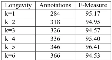
Another way to give users control over stopping behavior is to give them control over the longevity for which agreement (at the specified intensity) must be maintained before SP concludes to stop. The sim-plest implementation would be to check the most recent model with the previous model and stop if their agreement exceeds the intensity cutoff. How-ever, independent of wanting to provide users with a longevity control, this is not an ideal approach be-cause there’s a risk that these two models could hap-pen to highly agree but then the next model will not highly agree with them. Therefore, we propose us-ing the average of the agreements from a window of the k most recent pairs of models. If we call the most recent model Mn, the previous model Mn−1 and so on, with a window size of 3, we average the agreements betweenMnandMn−1, betweenMn−1 andMn−2, and betweenMn−2andMn−3. On sepa-rate development data a window size of k=3 worked well. All of the experiments (except those in Ta-ble 3) in the current paper used a longevity window

size of k=3 with zero tuning performed. We will see in Section 4 that this longevity default delivers robust results across all of the folds for all of the datasets. Furthermore, Section 4 shows that varying the longevity requirement provides users with an-other lever for controlling how aggressively SP will behave.

4 Evaluation and Discussion

4.1 Experimental Setup

We evaluate the Stabilizing Predictions (SP) stop-ping method on multiple datasets for Text Classifi-cation (TC) and Named Entity Recognition (NER) tasks. All of the datasets are freely and publicly available and have been used in many past works.

For Text Classification, we use two publicly avail-able spam corpora: the spamassassin corpus used in (Sculley, 2007) and the TREC spam corpus trec05p-1/ham25 described in (Cormack and Lynam, 2005). For both of these corpora, the task is a binary clas-sification task and we perform 10-fold cross valida-tion. We also use the Reuters dataset, in particular the Reuters-21578 Distribution 1.0 ModApte split2. Since a document may belong to more than one cat-egory, each category is treated as a separate binary classification problem, as in (Joachims, 1998; Du-mais et al., 1998). Consistent with (Joachims, 1998; Dumais et al., 1998), results are reported for the ten largest categories. Other TC datasets we use are the 20Newsgroups3newsgroup article classification and the WebKB web page classification datasets. For WebKB, as in (McCallum and Nigam, 1998; Zhu et al., 2008a; Zhu et al., 2008b) we use the four largest categories. For all of our TC datasets, we use binary features for every word that occurs in the training data at least three times.

For NER, we use the publicly available GENIA corpus4. Our features, based on those from (Lee et al., 2004), are surface features such as the words in

2

http://www.daviddlewis.com/resources/ testcollections/reuters21578

3_{We used the “bydate” version of the dataset downloaded}

from http://people.csail.mit.edu/jrennie/20Newsgroups/. This version is recommended since it makes cross-experiment com-parison easier since there is no randomness in the selection of train/test splits.

4

the named entity and two words on each side, suf-fix information, and positional information. We as-sume a two-phase model where boundary identifica-tion has already been performed, as in (Lee et al., 2004).

SVMs deliver high performance for the datasets we use so we employ SVMs as our base learner in the bulk of our experiments (maximum entropy models are used in Subsection 4.3). For selection of points to query, we use the approach that was used in (Tong and Koller, 2002; Schohn and Cohn, 2000; Campbell et al., 2000) of selecting the points that are closest to the current hyperplane. We use SVMlight (Joachims, 1999) for training the SVMs. For the smaller datasets (less than 50,000 examples in total), a batch size of 20 was used with an initial training set of size 100 and for the larger datasets (greater than 50,000 examples in total), a batch size of 200 was used with an initial training set of size 1000.

4.2 Main Results

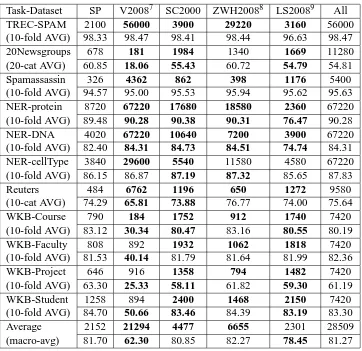
Table 1 shows the results for all of our datasets. For each dataset, we report the average number of anno-tations5 requested by each of the stopping methods as well as the average F-measure achieved by each of the stopping methods.6

There are two facts worth keeping in mind. First, the numbers in Table 1 are averages and therefore, sometimes two methods could have very similar average numbers of annotations but wildly differ-ent average F-measures (because one of the meth-ods was consistently stopping around its average whereas the other was stopping way too early and way too late). Second, sometimes a method with a higher average number of annotations has a lower

5

Better evaluation metrics would use more refined measures of annotation effort than the number of annotations because not all annotations require the same amount of effort to annotate but lacking such a refined model for our datasets, we use number of annotations in these experiments.

6_{Tests of statistical significance are performed using}

matched pairs t tests at a 95% confidence level. 7

(Vlachos, 2008) suggests using three drops in a row to de-tect a consistent drop in confidence so we do the same in our implementation of the method from (Vlachos, 2008).

8_{Following (Zhu et al., 2008b), we set the starting accuracy}

threshold to 0.9 when reimplementing their method.

9_{(Laws and Sch¨utze, 2008) uses a window of size 100}

and a threshold of 0.00005 so we do the same in our re-implementation of their method.

average F-measure than a method with a lower aver-age number of annotations. This can be caused be-cause of the first fact just mentioned about the num-bers being averages and/or this can also be caused by the ”less is more” phenomenon in active learn-ing where often with less data, a higher-performlearn-ing model is learned than with all the data; this was first reported in (Schohn and Cohn, 2000) and sub-sequently observed by many others (e.g., (Vlachos, 2008; Laws and Sch¨utze, 2008)).

There are a few observations to highlight regard-ing the performance of the various stoppregard-ing meth-ods:

• SP is the most parsimonious method in terms of annotations. It stops the earliest and remark-ably it is able to do so largely without sacrific-ing F-measure.

• All the methods except for SP and SC2000 are unstable in the sense that on at least one dataset they have a major failure, either stopping way too late and wasting large numbers of anno-tations (e.g. ZWH2008 and V2008 on TREC Spam) or stopping way too early and losing large amounts of F-measure (e.g. LS2008 on NER-Protein) .

• It’s not always clear how to evaluate stopping methods because the tradeoff between the value of extra F-measure versus saving annotations is not clearly known and will be different for dif-ferent applications and users.

This last point deserves some more discussion. In some cases it is clear that one stopping method is the best. For example, on WKB-Project, the SP method saves the most annotations and has the high-est F-measure. But which method performs the best on NER-DNA? Arguments can reasonably be made for SP, SC2000, or ZWH2008 being the best in this case depending on what exactly the anno-tation/performance tradeoff is. A promising direc-tion for research on AL stopping methods is to de-velop user-adjustable stopping methods that stop as aggressively as the user’s annotation/performance preferences dictate.

Task-Dataset SP V20087 SC2000 ZWH20088 LS20089 All

TREC-SPAM 2100 56000 3900 29220 3160 56000

(10-fold AVG) 98.33 98.47 98.41 98.44 96.63 98.47

20Newsgroups 678 181 1984 1340 1669 11280

(20-cat AVG) 60.85 18.06 55.43 60.72 54.79 54.81

Spamassassin 326 4362 862 398 1176 5400

(10-fold AVG) 94.57 95.00 95.53 95.94 95.62 95.63

NER-protein 8720 67220 17680 18580 2360 67220

(10-fold AVG) 89.48 90.28 90.38 90.31 76.47 90.28

NER-DNA 4020 67220 10640 7200 3900 67220

(10-fold AVG) 82.40 84.31 84.73 84.51 74.74 84.31

NER-cellType 3840 29600 5540 11580 4580 67220

(10-fold AVG) 86.15 86.87 87.19 87.32 85.65 87.83

Reuters 484 6762 1196 650 1272 9580

(10-cat AVG) 74.29 65.81 73.88 76.77 74.00 75.64

WKB-Course 790 184 1752 912 1740 7420

(10-fold AVG) 83.12 30.34 80.47 83.16 80.55 80.19

WKB-Faculty 808 892 1932 1062 1818 7420

(10-fold AVG) 81.53 40.14 81.79 81.64 81.99 82.36

WKB-Project 646 916 1358 794 1482 7420

(10-fold AVG) 63.30 25.33 58.11 61.82 59.30 61.19

WKB-Student 1258 894 2400 1468 2150 7420

(10-fold AVG) 84.70 50.66 83.46 84.39 83.19 83.30

Average 2152 21294 4477 6655 2301 28509

(macro-avg) 81.70 62.30 80.85 82.27 78.45 81.27

Table 1: Methods for stopping AL. For each dataset, the average number of annotations at the automatically determined stopping points and the average F-measure at the automatically determined stopping points are displayed. Bold entries are statistically significantly different than SP (and non-bold entries are not). The Average row is simply an unweighted macro-average over all the datasets. The final column (labeled ”All”) represents standard fully supervised passive learning with the entire set of training data.

too much while others are known to perform consis-tently in a conservative manner, then users can pick the stopping criterion that’s more suitable for their particular annotation/performance valuation. For this purpose, SP fills a gap as the other stopping cri-teria seem to be conservative in the sense defined in Section 1. SP, on the other hand, is more of an aggressive stopping criterion and is less likely to an-notate data that is not needed.

A second avenue for providing user-adjustable stopping is a single stopping method that is itself ad-justable. To this end, Section 4.3 shows how

inten-sity and longevity provide levers that can be used to

control the behavior of SP in a controlled fashion.

Sometimes viewing the stopping points of the

var-ious criteria on a graph with the active learning curve can help one visualize how the methods perform. Figure 2 shows the graph for a representative fold.10 The x-axis measures the number of human annota-tions that have been requested so far. The y-axis measures performance in terms of F-Measure. The vertical lines are where the various stopping meth-ods would have stopped AL if we hadn’t continued the simulation. The figure reinforces and illustrates what we have seen in Table 1, namely that SP stops more aggressively than existing criteria and is able

10

0 1 2 3 4 5 6 7

x 104

60 65 70 75 80 85 90

Number of Human Annotations Requested

Performance (F−Measure)

DNA Fold 1

SC2000

LS2008

ZWH2008 V2008 SP

Figure 2: Graphic with stopping criteria in action for fold 1 of NER of DNA from the GENIA corpus. The x-axis ranges from 0 to 70,000.

to do so without sacrificing performance.

4.3 Additional Experiments

All of the additional experiments in this subsection were conducted on our least computationally de-manding dataset, Spamassassin. The results in Ta-bles 2 and 3 show how varying the intensity cut-off and the longevity requirement, respectively, of SP enable a user to control stopping behavior. Both methods enable a user to adjust stopping in a con-trolled fashion (without radical changes in behav-ior). Areas of future work include: combining the intensity and longevity methods for controlling be-havior; and developing precise expectations on the change in behavior corresponding to changes in the intensity and longevity settings.

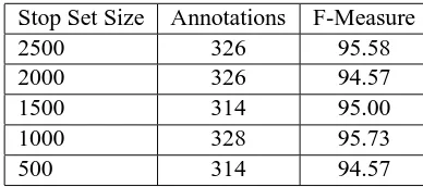
The results in Table 4 show results for different stop set sizes. Even with random selection of a stop set as small as 500, SP’s performance holds fairly steady. This plus the fact that random selection of stop sets of size 2000 worked across all the folds of all the datasets in Table 1 show that in practice per-haps the simple heuristic of choosing a fairly large random set of points works well. Nonetheless, we think the size necessary will depend on the dataset and other factors such as the feature representation so more principled methods of determining the size and/or the makeup of the stop set are an area for future work. For example, construction techniques

Intensity Annotations F-Measure

K=99.5 364 96.01

K=99.0 326 94.57

K=98.5 304 95.59

K=98.0 262 93.75

K=97.5 242 93.35

K=97.0 224 90.91

Table 2: Controlling the behavior of stopping through the use of intensity. For Kappa intensity levels in_{97.0, 97.5, 98.0, 98.5, 99.0, 99.5_}, the 10-fold average number of an-notations at the automatically determined stopping points and the 10-fold average F-measure at the automatically determined stopping points are displayed for the Spamas-sassin dataset.

Longevity Annotations F-Measure

k=1 284 95.17

k=2 318 94.95

k=3 326 94.57

k=4 336 95.40

k=5 346 96.41

k=6 366 94.53

Table 3: Controlling the behavior of stopping through the use of longevity. For window length k longevity levels in

{1, 2, 3, 4, 5, 6_}, the 10-fold average number of annota-tions at the automatically determined stopping points and the 10-fold average F-measure at the automatically deter-mined stopping points are displayed for the Spamassassin dataset.

accom-Task-Dataset SP V2008 ZWH2008 LS2008 All

Spamassassin 286 1208 386 756 5400

(10-fold AVG) 94.92 89.89 95.31 96.40 91.74

Table 5: Methods for stopping AL with maximum entropy as the base learner. For each stopping method, the average number of annotations at the automatically determined stopping point and the average F-measure at the automatically determined stopping point are displayed. Bold entries are statistically significantly different than SP (and non-bold entries are not). SC2000, the margin exhaustion method, is not shown since it can’t be used with a non-margin-based learner. The final column (labeled ”All”) represents standard fully supervised passive learning with the entire set of training data.

Stop Set Size Annotations F-Measure

2500 326 95.58

2000 326 94.57

1500 314 95.00

1000 328 95.73

500 314 94.57

Table 4: Investigating the sensitivity to stop set size. For stop set sizes in_{2500, 2000, 1500, 1000, 500_}, the 10-fold average number of annotations at the automatically determined stopping points and the 10-fold average F-measure at the automatically determined stopping points are displayed for the Spamassassin dataset.

plished by perhaps continuing to add examples to the stop set until adding new examples is no longer increasing the representativeness of the stop set.

As one of the advantages of SP is that it’s widely applicable, Table 5 shows the results when using maximum entropy models as the base learner dur-ing AL (the query points selected are those which the model is most uncertain about). The results re-inforce our conclusions from the SVM experiments, with SP performing aggressively and all statistically significant differences in performance being in SP’s favor. Figure 3 shows the graph for a representative fold.

5 Conclusions

Effective methods for stopping AL are crucial for re-alizing the potential annotation savings enabled by AL. A survey of existing stopping methods identi-fied three areas where improvements are called for. The new stopping method based on Stabilizing Pre-dictions (SP) addresses all three areas: SP is widely applicable, stable, and aggressive in saving annota-tions.

0 1000 2000 3000 4000 5000 6000

50 60 70 80 90 100

Number of Human Annotations Requested

Performance (F−Measure)

AL−MaxEnt: Spamassassin Fold 5

SP

ZWH2008

LS2008 V2008

Figure 3: Graphic with stopping criteria in action for fold 5 of TC of the spamassassin corpus. The x-axis ranges from 0 to 6,000.

References

Ron Artstein and Massimo Poesio. 2008. Inter-coder agreement for computational linguistics. Computa-tional Linguistics, 34(4):555–596.

Jason Baldridge and Miles Osborne. 2008. Active learn-ing and logarithmic opinion pools for hpsg parse se-lection. Nat. Lang. Eng., 14(2):191–222.

Michael Bloodgood and K. Vijay-Shanker. 2009. Taking into account the differences between actively and pas-sively acquired data: The case of active learning with support vector machines for imbalanced datasets. In

NAACL.

Colin Campbell, Nello Cristianini, and Alex J. Smola. 2000. Query learning with large margin classifiers. In ICML ’00: Proceedings of the Seventeenth

Interna-tional Conference on Machine Learning, pages 111–

118, San Francisco, CA, USA. Morgan Kaufmann Publishers Inc.

J. Cohen. 1960. A coefficient of agreement for nominal scales. Educational and Psychological Measurement, 20:37–46.

Gordon Cormack and Thomas Lynam. 2005. Trec 2005 spam track overview. In TREC-14.

Susan Dumais, John Platt, David Heckerman, and Mehran Sahami. 1998. Inductive learning algorithms and representations for text categorization. In CIKM

’98: Proceedings of the seventh international con-ference on Information and knowledge management,

pages 148–155, New York, NY, USA. ACM.

Seyda Ertekin, Jian Huang, L´eon Bottou, and C. Lee Giles. 2007. Learning on the border: active learn-ing in imbalanced data classification. In M´ario J. Silva, Alberto H. F. Laender, Ricardo A. Baeza-Yates, Deborah L. McGuinness, Bjørn Olstad, Øystein Haug Olsen, and Andr´e O. Falc˜ao, editors, Proceedings of

the Sixteenth ACM Conference on Information and Knowledge Management, CIKM 2007, Lisbon, Portu-gal, November 6-10, 2007, pages 127–136. ACM.

Thorsten Joachims. 1998. Text categorization with su-port vector machines: Learning with many relevant features. In ECML, pages 137–142.

Thorsten Joachims. 1999. Making large-scale SVM learning practical. In Advances in Kernel Methods –

Support Vector Learning, pages 169–184.

Florian Laws and Hinrich Sch ¨utze. 2008. Stopping crite-ria for active learning of named entity recognition. In

Proceedings of the 22nd International Conference on Computational Linguistics (Coling 2008), pages 465–

472, Manchester, UK, August. Coling 2008 Organiz-ing Committee.

Ki-Joong Lee, Young-Sook Hwang, Seonho Kim, and Hae-Chang Rim. 2004. Biomedical named entity

recognition using two-phase model based on svms.

Journal of Biomedical Informatics, 37(6):436–447.

Andrew McCallum and Kamal Nigam. 1998. A compar-ison of event models for naive bayes text classification. In Proceedings of AAAI-98, Workshop on Learning for

Text Categorization.

Greg Schohn and David Cohn. 2000. Less is more: Ac-tive learning with support vector machines. In Proc.

17th International Conf. on Machine Learning, pages

839–846. Morgan Kaufmann, San Francisco, CA. D. Sculley. 2007. Online active learning methods for fast

label-efficient spam filtering. In Conference on Email

and Anti-Spam (CEAS), Mountain View, CA, USA.

Simon Tong and Daphne Koller. 2002. Support vec-tor machine active learning with applications to text classification. Journal of Machine Learning Research

(JMLR), 2:45–66.

Andreas Vlachos. 2008. A stopping criterion for active learning. Computer Speech and Language, 22(3):295– 312.

Jingbo Zhu and Eduard Hovy. 2007. Active learning for word sense disambiguation with methods for ad-dressing the class imbalance problem. In Proceedings

of the 2007 Joint Conference on Empirical Methods in Natural Language Processing and Computational Natural Language Learning (EMNLP-CoNLL), pages

783–790.

Jingbo Zhu, Huizhen Wang, and Eduard Hovy. 2008a. Learning a stopping criterion for active learning for word sense disambiguation and text classification. In

IJCNLP.

Jingbo Zhu, Huizhen Wang, and Eduard Hovy. 2008b. Multi-criteria-based strategy to stop active learning for data annotation. In Proceedings of the 22nd

Interna-tional Conference on ComputaInterna-tional Linguistics (Col-ing 2008), pages 1129–1136, Manchester, UK,