Abstract— Recurrent neural networks (RNN) are a class of densely connected single layer nonlinear networks of perceptrons. The network’s energy function is defined through a learning procedure so that its minima coincide with states from a predefined set. . However, because of the network’s nonlinearity a number of undesirable local energy minima emerge from the learning procedure. This has shown to significantly effect the network’s performance. In this work we analyze the rate of convergence for three iterative procedures namely- Mann, Ishikawa and J-iterations in recurrent network and many important results have been worked out for decreasing as well as increasing functions. The results obtained are very useful for designing of inner product kernel of support vector machine with faster convergence rate.
Index Terms—Stable States, Mann Iteration, Ishikawa Iterations, J-Iteration, Convergence
I. INTRODUCTION
Neural networks are a class of non-linear function approximators. It is originated by McCulloch and Pitt [1], Hebb[2], and Rosenblatt[3][4]. Hopfield defined a single-layer network consisting of interconnected individual perceptrons and modified perceptrons (with sigmoidal non-linearties) [5][6][7]. The basis for network operation as a content addressable memory is the Hebbian learning algorithm. The idea is to choose network connections in a way that the energy function associated with the network can be minimized for a set of desired network states. Unfortunately, because of its nonlinear character, the network has also exhibited non-desirable, local minima. This has shown to affect the network performance, both in its capacity and its ability to address its content [8][9][10]. Several approaches based on simulated annealing and other techniques have been proposed that deal with the problem of local minima [11][12][13][14][15][16]. In these approaches, an inherent assumption of the final network state (Gibbs) distribution is proposed. The motivation for these assumptions is that the Gibbs distribution provides a mechanism for the characterization of the global minima. In many applications, such as neural networks, however, the
Manuscript received October 9, 2009. This work was supported by the Birla Institute of Technology, Allahabad Campus, Allahabad (UP), India.
Subhash Chandra Pandey is with the Birla Institute of Technology,Allahabad Campus, Allahabad(UP), India phone: +91-532-2687363;( e-mail: [email protected]).
Prof. G.C. Nandi is with Indian Institute of Information Technology, Allahabad-211012(UP), India. His research interests includes Soft computing, Artificial Intelligence, Robotics and Industrial automation, Advanced Artificial Intelligence, Computer Controlled Systems, Humanoid robots , Machine vision and processing.
desired final network state distribution corresponds to particular local minima, and not necessarily to the global minima. The use of Gibbs distribution is thus undesirable in many applications. A modification of this approach can be used to enhance the performance of neural networks. In this work we have compared the number of iterations
required to achieve the stable state in recurrent auto associative neural networks for the three iterative processes i.e. Mann, Ishikawa and J-iteration. The paper is organized as follows: In section II we introduced some preliminaries and definitions regarding the Mann, Ishikawa and J-iterative processes. In section III we relate the memory convergence concept in recurrent autoassociative neural network. Section IV describes the detailed experimental output obtained pertaining to these iterative processes. This is followed by applications in section V and concluding remarks are given in VI.
II. PRELIMINARIES
In this section, we will discuss the basic concepts related to Mann, Ishikawa and J-iterations.
Let T : X → X be a self mapping and (X,d) be a metric linear space. The three iterative processes are defined as:
Definition2.1: Let A be a lower triangular matrix with nonnegative entries and it is defined that Zn+1 =T(Vn) , where
V
n=
∑
a
nkZ
k .The Mann iterative process is obtained by choosing a sequence{
α
n}
which satisfy (1)1
0
=
α
(2)0
≤
α
n<
1
forn
>
0
and (3)∑
α
n=
∞
.Then the entries of A become
a
nn=
α
n ,a
nk=
α
k∏
(
1
−
α
i),
k
<
n
. The above representationof
A
leads the following form:n n n n
n
Z
TZ
Z
+1=
(
1
−
α
)
+
α
. It should be noted that forα
n=
1
, this form reduces to the Picard iterative process i.e.Z
n+1=
TZ
n.Definition2.2: The Ishikawa iterative procedure is defined
as- Let
x
0∈
X
,n n n n n
n n n n
n
X
Ty
y
X
TX
X
+1=
(
1
−
α
)
+
α
,
=
(
1
−
β
)
+
β
,n
>
0
, where{
α
n}
,
{
β
n}
are sequences of positive numbers. They also satisfy the conditions (1)0
≤
α
n≤
β
n≤
1
(2)0
lim
β
n=
and (3)∑
α
nβ
n=
∞
. In [18] the inequalityMemory Convergence Analysis for Different
Iterative Procedures in RNN
condition has been replaced by
0
≤
α
n andβ
n≤
1
and thus broaden the class of Ishikawa process. It also helps to reduce it to the Mann process by settingβ
n=
0
. In spite ofthis similarity, however, there is no any resemblance in convergence of these methods.
Definition2.3:The Jungck iterative procedure is commonly known as J-iterative procedure. It is defined as.
For
S
:
X
→
X
,
T
(
X
)
⊆
S
(
X
),
x
0∈
X
,
SX
n+1=
TX
n,
n
=
0
,
1
,....
It is worthwhile to mention that if
S
is the identity map onX
, this procedure will be reduce to the Picard iteration. In [17], various applications of J-iterative procedures have been discussed in numerical praxis.Theorem2.4: Let S,T[a,b]→[a,b] be differentiable withSa ≠ Sb . Let
T
'
X
and S'X both are equal to zero for any x∈] [
a,b . Then the pair (S,T) is said to be J-contraction of[
a
,
b
]
if and only if there exists a positive numberq
<
1
such that T'y ≤ qS'y for all y∈] [
a,b .Let
{
X
n}
be a sequence generated by an iterative procedure f(T,Xn)of the neural network that converges to a stable state ofT
. It is important to mention that for any mapT
, the initial choice x0 determines the stable state ofT
where the sequence
{
X
n}
will converge. Thus, ifT
is non-decreasing with three distinct stable statesp
,
q
,
r
and satisfies the conditions0
≤
p
<
q
<
r
≤
1
, then) , 0 [ q
Xo∈ implies thatXn → p where as X0∈(q,1] impliesX n → r . The stable states
p
andr
are known as the attractive global minima whereasq
is a repulsive global minima. The sequence{
X
n}
will not converge to the unstable stateq
unless and untilX0 = q [18].If
{
X
n}
and{
Z
n}
are two iteration schemes which converge to the same global minimap
, then{
X
n}
is better than {Zn} if Xn − p ≤ Zn − p for alln
i.e.}
{Xn converges to
p
faster than{Zn}. This allows us to compare the rate of convergence of two iterative schemes.III. MEMORY CONVERGENCE CONCEPT
We now look in more detail at the convergence of recurrent auto associative networks. Since the energy functionE(X ) is bounded from below, the network evolves under the asynchronous dynamics towardE(X n+1) such that
E
(
X
n+1)
≤
E
(
X
n)
(1) It should be noted that vectorX
n+1andX
n differ during the memory transitions by at most a single component, the stabilization ofE(X n+1) means thatE(Xn+1)= E(Xn)
For
n
>
n
0 (2)The transition stop at the energy minimum, which also implies that
X
n+1=X
n (3) Thus the network reaches its stable stateX
n , at the energy minimumE
(
X
n)
. It is also obvious from energy function study that the only attractors of the discussed network are its stable states.
Let us begin with a one-dimensional recurrent system. For the output at
t
=
n
+
1
we have
X
n+1=f
(
w
,
X
n)
(4) The stable state is defined at *X if the following relationship holds:
X* = f(X*) (5) Where it has been assumed that network parameter
w
in equation (4) is constant. In geometrical terms the global minima is found at the intersection of function f(X)and
X
. In terms of the recursive formula (4), the global minima is said to be stable if
*
lim
X
nX
n→∞
=
(6)
Or
lim
+1=
0
∞→
n
n
e
. (7) Wheree
is the recursion error which can be defined as 1 1 *X X
en+ ≅ n+ −
The recursion error can be expressed using equation (4) as
1 *
)
(X X
f
en+ = n − (8)
and further rearranged to the form
n n n
n
e X X X f X X X f
e +1= [ { *+( − *)}− ( * )]/( − * (9)
It is obvious that for a differentiable function
f
responsible for network’s feed forward processing, this further reduces to en+1 ≅ f'(X *)en(10)
Now the condition (10) translates to the form
f'(X *) <1 (11)
This is sufficient condition for the existence of stable global minima in the neighborhood where condition (11) holds [19].
IV. EXPERIMENTS
of Mann and Ishikawa iteration exhibit interesting results. We programmed both schemes for the
functions m
X X
f( ) = (1− ) , for
m
=7, 8… 29, taking initial choiceX
0 = 0.9 andα
n=
β
n=
(
n
+
1
)
−1/2. It isobserved that in each case, the Mann process converges to a stable state (accurate to eight places) in 9-12 iterations whereas the Ishikawa method requires 38-42 iterations for the same accuracy.
In this section, we will continue this computational study and find the stable states of
h
andp
given below.Problem1.
h
(
X
)
=
(
1
−
X
)
m,m
= 7,8,……,29 Problem2. ( ) = 2 3 −7 2 +8 − 2X X X X
p
First, we consider problem 1 and developed a computer program for Mann iterative procedure whose inputs are the initial guess X0 and a value of
m
. The execution of program form
=7,X
0 = 0.9 and 1/2) 1 ( + − = n
n
α yield
the results listed in table I.
Further, a program is developed to solve the same problem using Ishikawa iterative procedure. The program is executed taking m=7, x0 = 0.9 and αn = βn = (n+1)-1/2 and results are listed in the table II.
Now, in order to solve the equation using J-iterative process, it is rewritten in the form of f(X) = g(X)
as f (X ) = X and
g
(
X
)
=
(
1
−
X
)
7. It should be notedthat the image of
g
is contained in the imagef
. Further, )( ' 1 ) 1 ( 7 ) (
' X X 6 f X
g = − ≤ = for
X
∈[0.2,0.9]. [image:3.595.304.521.58.541.2]Considering these f and
g
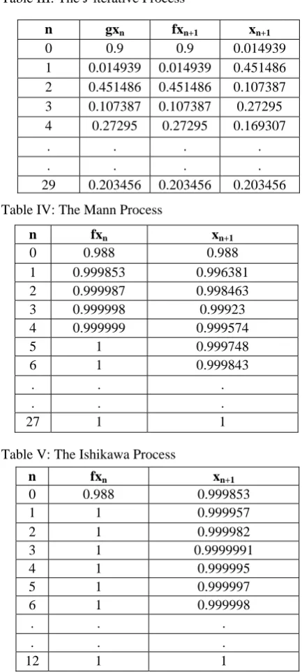
, again program is developed whose input is the initial guessX0 . The program is executed taking X0 = 0.9 and the reading are recorded in the table III. Table I: The Mann ProcessTable II: The Ishikawa Process
Table III: The J-iterative Process
Table IV: The Mann Process
Table V: The Ishikawa Process
Following the same method, programs are developed to
solve the problem 2 i.e. p(X) = 2X 3 −7X 2 +8X −2 ,
0
X =0.9 for Mann
and Ishikawa processes. The readings are listed in table IV and V.
Now a program is developed to solve problem 2 using J-iterative process taking
2
8
7
2
)
(
X
=
X
3−
X
2+
X
−
f
, andg
(
X
)
=
7
X
2 .The outputs of program for X0 = 0.9 are given in table VI. In order to provide a detailed study, these programs are again executed changing the parameters such as X0 = 0.2,
m
= 29 andα
n=
β
n=
(
n
+
1
)
−1/4 in problem 1 andX
0 = 0.6 andα
n=
β
n=
(
n
+
1
)
−1/4in problem 2.n fxn xn+1
0 1e-07 1e-07
1 0.999999 0.70706
2 0.000185 0.298965
3 0.08321 91088
4 0.226626 0.206981
. . . . . .
17 0.203456 0.203456
n fxn xn+1
0 1e-07 0.999999
1 8.235413e-4 4
0.355393
2 0.046245 0.2979776
3 0.084036 0.262381
4 0.118802 0.24034
. . . . . .
29 0.203456 0.203456
n gxn fxn+1 xn+1
0 0.9 0.9 0.014939
1 0.014939 0.014939 0.451486 2 0.451486 0.451486 0.107387 3 0.107387 0.107387 0.27295
4 0.27295 0.27295 0.169307
. . . . . . . . 29 0.203456 0.203456 0.203456
n fxn xn+1
0 0.988 0.988
1 0.999853 0.996381
2 0.999987 0.998463
3 0.999998 0.99923
4 0.999999 0.999574
5 1 0.999748
6 1 0.999843
. . .
. . .
27 1 1
n fxn xn+1
0 0.988 0.999853
1 1 0.999957
2 1 0.999982
3 1 0.9999991
4 1 0.999995
5 1 0.999997
6 1 0.999998
. . .
. . .
[image:3.595.39.243.478.783.2]Table VI: The J-iterative Process
The experiments have been repeated by taking different parameters and it is observed that for the decreasing functionh(X) = (1− X)m, for
m
=7 and0
X =0.9, the
Mann process converges to a stable state in 17th iteration, the Ishikawa in 29th iteration and J-iterative in 29th iteration (Table I, II, III). Similarly, for
m
=29 and X0=0.9, the Mann and Ishikawa iterative processes take 10 and 32 iterations respectively whereas J-iteration takes only15 iterations to converge to a stable state. It is also noted that when X0 =0.2 i.e. nearer to stable state, the number ofiterations for Mann, Ishikawa and J-processes are 7, 30 and 16 respectively. Moreover, when
α
n=
β
n=
(
n
+
1
)
−1/4 .We obtain the stable state in 17 and 45 iterations for Mann and Ishikawa. It has also been observed that when
α
n =1 i.e. Picard process the result is an oscillating sequence consisting of 0 and 1.The experiments revealed interesting facts for increasing function p(X) = 2X 3 −7X 2 +8X −2 when X0 = 0.9, the number of iterations required for Mann and Ishikawa are 27 and 12 respectively whereas J-iteration requires 165 iterations (Table IV, V, VI). It is also observed that when the initial guess is away from the stable states e.g. X0 = 0.6, we
get the stable states in just 5 iterations for all the three processes. Similarly, for
α
n=
β
n=
(
n
+
1
)
−1/4, the Mann process takes 9 iterations while the Ishikawa process takes only 5 iterations to convergence to a stable state. It is worth mentioning that forX
0 = 0.5 or 2, all the three processes converge toX
0 itself, but when 0.5< X0 <2, then{Xn}in all the three cases converge to 1.Further, whenn
α
=1 in algorithm, the result is obtained just in two iterations.
V. APPLICATIONS
In this section, we will describe the engineering application domain of our work. The results obtained in this work possess multifaceted real-life applications but here emphasis is given on support vector machine. Support vector machine is a learning machine and was initially designed to deal with binary classification with their linear decision functions. A support vector machine first maps the input points in to a high dimensional feature space and then finds a separating hyperplane that maximizes the margin between two classes in this feature space. Without any knowledge of mapping, the SVM uses kernels as the dot product functions in feature space. The solution of the optimal hyperplane can be written as a combination of a few input points called support vectors. The important types of support vector machines are: (1) Polynomial learning machine and the inner product kernel K(X ,X i),i =1,2,..., N for this SVM is(XTXi +1), where
p
is specified a priori by the user (2)Radial-basis function network , the kernel for RBF is defined as
⎟ ⎠ ⎞ ⎜
⎝ ⎛− −
=
2 2
2 1
i
x x e
y σ . The width
σ
2 , common to all the kernels, is specified as priori by the user (3) Two-layer perceptron for which the inner product kernel is)
tanh(
β
0+
β
1=
T ix
x
y
, and (4) Gaussian, for which theinner product kernel is 2
2
2 ) (
2
2
1 σ
πσ
a x
e y
− −
= . The detail
study of support vector machine is beyond the scope of this paper. For in-depth study of SVM, interested readers are requested to refer [20]. The results obtained in this work can be used for designing the inner product kernel with higher convergence rate. We can consider it as future work of this paper.
0 2 4 6 8 10 12 14 16 18 20 0
2 4 6 8 10 12 14 16 18
x 1012
x Radial Basis Function
y
Fig (1) Learning curve for Radial-Basis Function
n fxn fyn xn+1
0 5.758 5.758 0.9069
57 1 5.84077
5
5.84077 5
0.9134 53 2 5.91853
5
5.91853 5
0.9195 13 3 5.99150
1
5.99150 1
0.9251 64 4 6.05989
8
6.05989 8
0.9304 3
. . . .
. . . .
165 6.99999 4
6.99999 4
0 2 4 6 8 10 12 14 16 18 20 0.995
0.996 0.997 0.998 0.999 1 1.001
x y
Two Layer Perceptron
Fig (2) Learning curve for Two-Layer Perceptron
Fig (3) Learning curve for Polynomial SVM
0 2 4 6 8 10 12 14 16 18 20 0
0.02 0.04 0.06 0.08 0.1 0.12 0.14 0.16 0.18 0.2
x y
Gaussian
Fig (4) Learning curve for Gaussian SVM
VI. CONCLUSION
In this paper we analyze and compare the convergence rate for three iterative processes. For decreasing functions it has been concluded that for all combinations of
0
X ,
m
,α
n and nβ
, the decreasing order of rate of convergence of iterative procedures is: Mann, J-iterations and Ishikawa. On increasing the value ofm
, the Mann and Ishikawa processes require more number of iterations while J-iterative process requires less number of iterations to locate the stable state. For the initial guess nearer to the stable state, the Ishikawa scheme shows an increasing tendency whereas theJ-iterations have decreasing tendency in number of iterations but the Mann process shows no change. Indeed, the speed of iterative procedures depend on the position of {
α
n} and {β
n} in the interval (0, 1). Ifα
n andβ
n are larger, the stable state is obtained in more number of iterations for both Mann and Ishikawa scheme.It has also been worked out that for increasing functions for all combinations of
0
X ,
α
n andβ
n, the decreasing order of rate of convergence of iterative processes are: Ishikawa, Mann and J-iterations. If the initial guess is away from the stable state, the number of iterations increases in each of the three processes. It explicitly indicates that if initial guess is closer to the stable state, the results will be obtained quickly. Similarly, larger values ofα
nandβ
n, produces the results quickly for the Mann and Ishikawa process. The Picard iterative procedure i.e.α
n = 1is the best process for the approximation of stable state in increasing function. Most importantly, we may use the results obtained in this work for the design of inner-product kernelK(X ,Xi)ofsupport vector machine to construct the optimal hyperplane in the feature space without having to consider the feature space itself in explicit form.
REFERENCES
[1] W.McCulloch and W.Pitts. “Alogical calculus of the ideas imminent in nervous activity,” Bulletin of Mathematical Biophysics, vol 5, pp. 115-133, 1943.
[2] D.Hebb,The Organization of Behavior, New York, New York, John Wiley and Sons, 1949
[3] R. Rosenblatt, “The perceptron: A probabilistic model for information storage and organization in the brain, “Psychological Review”, vol65, pp.386-408, 1958.
[4] R. Rosenblatt Principles of Neurodynamics, New York, New York: Spartan Books, 1959.
[5] J. Hopfield, “Neural Network and Physical Systems with Emergent Collective Computational Abilities,” Proceedings of the Neural Academy of Science .USA, vol 79, pp. 2554-2558, April1982. [6] J. Hopfield, “Neurons with Graded Response Have Collective
Computational Properties like Those of Two-State Neurons,” Proceedings of the Neural Academy of Science .USA, vol81, pp. 3088-3092.
[7] J. Hopfield and D. Tank, “Computing with Neural Circuits: A Model,” Science, vol 233, pp. 625-633, 1986.
[8] S. Amari, “learning Pattern and Pattern sequence by Self-Organizing Nets of Threshold Elements,”IEEE Transaction on Computers, vol. C-21, no. 11, pp. 1197-1206.
[9] S. Amari and K. Maginu, “Statistical Neurodynamics of Associative Memory,” Neural Networks,vol 1, pp. 63-73, 1988.
[10] R. Lippmann, “An introduction to Computing with Neural Net,” IEEE Acoustics, Speech and Signal Processing Magazine,pp. 4-22,April 1987.
[11] S. Venkatesh and D. Psatis, “On Reliable Computations with Formal Neurons,” IEEE Transactions on Pattern Analysis and Machine Intelligence, vol. 14, no. 1, pp. 87-91, January 1992.
[12] I. Arizono, A. Yamamoto, and H. Ohta, “Scheduling for Minimizing total actual flow time by neural networks,” International Journal of Production Research, vol. 30, no.3, pp. 503-511, March 1992. [13] B. Lee and B. Sheu, “Modified Hopfield Neural Networks for
Retrieving the Optimal Solution,” IEEE Transaction on Neural Networks. vol. 2, no. 1, pp. 137-142, January 1991.
[14] M. Lu, Y. Zhan, and G. Mu, “Bipolar Optical Neural Networks with Adaptive Threshold,” Optik. Vol. 91, no 4, pp. 178-182, 1992.
0 2 4 6 8 10 12 14 16 18 20 0
2 4 6 8 10 12 14 16 18x 10
4
x y
[15] S.L. Lin, J.M. Wu, an C.Y. Liou, “ Annealing by Perturbing Synapses,” IEICE Transactions on Information and Systems, vol. E75-D, no. 2, pp. 210-218, March 1992.
[16] E. Wong, “Stochastic Neural Networks,” Algorithmica, pp. 466-478, June 1991.
[17] S.L. Singh, “Anew approach in numerical praxis,” Prog. Math. 32 (2), pp. 75-89, 1998.
[18] B. E. Rhoades, “Comment on two fixed point iteration methods,”J.Math. Anal. Appl.56, pp. 741-750.
[19] Jacek M. Zurada, “Introduction to Artificial Neural System”,jaico publication, pp.349-350,2002.