Learning to Generate Compositional Color Descriptions
Will Monroe,1 Noah D. Goodman,2 and Christopher Potts3
Departments of1Computer Science,2Psychology, and3Linguistics Stanford University, Stanford, CA 94305
[email protected], {ngoodman,cgpotts}@stanford.edu
Abstract
The production of color language is essential for grounded language generation. Color de-scriptions have many challenging properties: they can be vague, compositionally complex, and denotationally rich. We present an effec-tive approach to generating color descriptions using recurrent neural networks and a Fourier-transformed color representation. Our model outperforms previous work on a conditional language modeling task over a large corpus of naturalistic color descriptions. In addition, probing the model’s output reveals that it can accurately produce not only basic color terms but also descriptors with non-convex denota-tions (“greenish”), bare modifiers (“bright”, “dull”), and compositional phrases (“faded teal”) not seen in training.
1 Introduction
Color descriptions represent a microcosm of grounded language semantics. Basic color terms like “red” and “blue” provide a rich set of seman-tic building blocks in a continuous meaning space; in addition, people employ compositional color de-scriptions to express meanings not covered by ba-sic terms, such as “greenish blue” or “the color of the rust on my aunt’s old Chevrolet” (Berlin and Kay, 1991). The production of color language is essential for referring expression generation (Krah-mer and Van Deemter, 2012) and image captioning (Kulkarni et al., 2011; Mitchell et al., 2012), among other grounded language generation problems.
We consider color description generation as a grounded language modeling problem. We present
Color Top-1 Sample
(83, 80, 28) “green” “very green”
(232, 43, 37) “blue” “royal indigo”
(63, 44, 60) “olive” “pale army green” (39, 83, 52) “orange” “macaroni”
Table 1: A selection of color descriptions sampled from our model that were not seen in training. Color triples are in HSL. Top-1shows the model’s highest-probability prediction.
an effective new model for this task that uses a long short-term memory (LSTM) recurrent neural net-work (Hochreiter and Schmidhuber, 1997; Graves, 2013) and a Fourier-basis color representation in-spired by feature representations in computer vision. We compare our model with LUX (McMahan and Stone, 2015), a Bayesian generative model of color semantics. Our model improves on their approach in several respects, which we demonstrate by exam-ining the meanings it assigns to various unusual de-scriptions: (1) it can generate compositional color descriptions not observed in training (Fig. 3); (2) it learns correct denotations for underspecified modi-fiers, which name a variety of colors (“dark”, “dull”; Fig. 2); and (3) it can model non-convex denota-tions, such as that of “greenish”, which includes both greenish yellows and blues (Fig. 4). As a result, our model also produces significant improvements on several grounded language modeling metrics.
2 Model formulation
Formally, a model of color description generation is a probability distributionS(d|c)over sequences of
c
<s> light blue </s> light blue
LSTM FC softmax
c
light blue
FC FC softmax
f f f f
[image:2.612.100.270.56.159.2]d0 d1 d2
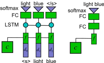
Figure 1: Left: sequence model architecture; right: atomic-description baseline. FC denotes fully connected layers.
tokensdconditioned on a colorc, wherecis
repre-sented as a 3-dimensional real vector in HSV space.1
Architecture Our main model is a recurrent neu-ral network sequence decoder (Fig. 1, left panel). An input color c = (h, s, v) is mapped to a
rep-resentationf (see Color features, below). At each
time step, the model takes in a concatenation off
and an embedding for the previous output tokendi,
starting with the start tokend0 = <s>. This
con-catenated vector is passed through an LSTM layer, using the formulation of Graves (2013). The out-put of the LSTM at each step is passed through a fully-connected layer, and a softmax nonlinearity is applied to produce a probability distribution for the following token.2 The probability of a sequence is the product of probabilities of the output tokens up to and including the end token</s>.
We also implemented a simple feed-forward neu-ral network, to demonstrate the value gained by modeling descriptions as sequences. This architec-ture (atomic; Fig. 1, right panel) consists of two fully-connected hidden layers, with a ReLU nonlin-earity after the first and a softmax output over all full color descriptions seen in training. This model therefore treats the descriptions as atomic symbols rather than sequences.
Color features We compare three representations:
• Raw: The original 3-dimensional color vectors, in HSV space.
1HSV: hue-saturation-value. The visualizations and tables
in this paper instead use HSL (hue-saturation-lightness), which yields somewhat more intuitive diagrams and differs from HSV by a trivial reparameterization.
2Our implementation uses Lasagne (Dieleman et al., 2015),
a neural network library based on Theano (Al-Rfou et al., 2016).
• Buckets: A discretized representation, dividing HSV space into rectangular regions at three res-olutions (90×10×10, 45×5×5, 1×1×1) and assigning a separate embedding to each region. • Fourier: Transformation of HSV vectors into a Fourier basis representation. Specifically, the representationf of a color(h, s, v)is given by
ˆ
fjk` = exp [−2πi(jh∗+ks∗+`v∗)]
f =Re{fˆ} Im{fˆ} j, k, `= 0..2
where(h∗, s∗, v∗) = (h/360, s/200, v/200).
The Fourier representation is inspired by the use of Fourier feature descriptors in computer vision appli-cations (Zhang and Lu, 2002). It is a nonlinear trans-formation that maps the 3-dimensional HSV space to a 54-dimensional vector space. This representa-tion has the property that most regions of color space denoted by some description are extreme along a single direction in Fourier space, thus largely avoid-ing the need for the model to learn non-monotonic functions of the color representation.
Training We train using Adagrad (Duchi et al., 2011) with initial learning rateη=0.1, hidden layer
size and cell size 20, and dropout (Hinton et al., 2012) with a rate of 0.2 on the output of the LSTM and each fully-connected layer. We identified these hyperparameters with random search, evaluating on a held-out subset of the training data.
We use random normally-distributed initialization for embeddings (σ =0.01) and LSTM weights (σ=
0.1), except for forget gates, which are initialized to a constant value of 5. Dense weights use normalized uniform initialization (Glorot and Bengio, 2010).
3 Experiments
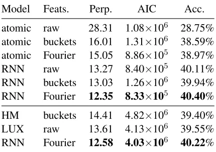
We demonstrate the effectiveness of our model us-ing the same data and statistical modelus-ing metrics as McMahan and Stone (2015).
Model Feats. Perp. AIC Acc. atomic raw 28.31 1.08×10⁶ 28.75%
atomic buckets 16.01 1.31×10⁶ 38.59%
atomic Fourier 15.05 8.86×10⁵ 38.97%
RNN raw 13.27 8.40×10⁵ 40.11%
RNN buckets 13.03 1.26×10⁶ 39.94%
RNN Fourier 12.35 8.33×10⁵ 40.40%
HM buckets 14.41 4.82×10⁶ 39.40%
LUX raw 13.61 4.13×10⁶ 39.55%
[image:3.612.78.293.59.210.2]RNN Fourier 12.58 4.03×10⁶ 40.22%
Table 2:Experimental results. Top: development set; bottom: test set. AIC is not comparable between the two splits. HM and LUX are from McMahan and Stone (2015). We reimplemented HM and re-ran LUX from publicly available code, confirming all results to the reported precision except perplexity of LUX, for which we obtained a figure of 13.72.
very rarely. The resulting dataset contains 2,176,417 pairs divided into training (1,523,108), development (108,545), and test (544,764) sets.
Metrics We quantify model effectiveness with the following evaluation metrics:
• Perplexity: The geometric mean of the recip-rocal probability assigned by the model to the descriptions in the dataset, conditioned on the respective colors. This expresses the same ob-jective as log conditional likelihood. We follow McMahan and Stone (2015) in reporting per-plexity per-description, not per-token as in the language modeling literature.
• AIC: The Akaike information criterion (Akaike, 1974) is given by AIC = 2`+ 2k,
where ` is log likelihood and k is the total
number of real-valued parameters of the model (e.g., weights and biases, or bucket proba-bilities). This quantifies a tradeoff between accurate modeling and model complexity. • Accuracy: The percentage of most-likely
de-scriptions predicted by the model that exactly match the description in the dataset (recall@1).
Results The top section of Table 2 shows devel-opment set results comparing modeling effective-ness for atomic and sequence model architectures
and different features. The Fourier feature transfor-mation generally improves on raw HSV vectors and discretized embeddings. The value of modeling de-scriptions as sequences can also be observed in these results; the LSTM models consistently outperform their atomic counterparts.
Additional development set experiments (not shown in Table 2) confirmed smaller design choices for the recurrent architecture. We evaluated a model with two LSTM layers, but we found that the model with only one layer yielded better perplexity. We also compared the LSTM with GRU and vanilla re-current cells; we saw no significant difference be-tween LSTM and GRU, while using a vanilla recur-rent unit resulted in unstable training. Also note that the color representationfis input to the model at
ev-ery time step in decoding. In our experiments, this yielded a small but significant improvement in per-plexity versus using the color representation as the initial state.
Test set results appear in the bottom section. Our best model outperforms both the histogram baseline (HM) and the improved LUX model of McMahan and Stone (2015), obtaining state-of-the-art results on this task. Improvements are highly significant on all metrics (p <0.001, approximate permutation
test,R=10,000 samples; Padó, 2006).
4 Analysis
Given the general success of LSTM-based mod-els at generation tasks, it is perhaps not surprising that they yield good raw performance when applied to color description. The color domain, however, has the advantage of admitting faithful visualiza-tion of descripvisualiza-tions’ semantics: colors exist in a 3-dimensional space, so a two-3-dimensional visualiza-tion can show an acceptably complete picture of an entire distribution over the space. We exploit this to highlight three specific improvements our model realizes over previous ones.
We construct visualizations by querying the model for the probabilityS(d | c) of the same
0 20 40 60 80 100 Li gh tn ess
0 20 40 60 80 100 Saturation "light" 0 20 40 60 80 100 Li gh tn ess
0 20 40 60 80 100 Saturation "bright" 0 20 40 60 80 100 Li gh tn ess
0 20 40 60 80 100 Saturation "dark" 0 20 40 60 80 100 Li gh tn ess
[image:4.612.83.286.56.262.2]0 20 40 60 80 100 Saturation "dull"
Figure 2:Conditional likelihood of bare modifiers according to our generation model as a function of color. White represents regions of high likelihood. We omit the hue dimension, as these modifiers do not express hue constraints.
Formally, each visualization is a pair of functions
(L, R), where
L(s, `) = log
R
dh S(d|c= (h, s, `))
R
dc0 S(d|c0)
R(h, `) = log
R
ds S(d|c= (h, s, `))
R
dc0 S(d|c0)
The maximum value of each function is plotted as white, the minimum value is black, and intermediate values linearly interpolated.
[image:4.612.322.522.57.281.2]Learning modifiers Our model learns accurate meanings of adjectival modifiers apart from the full descriptions that contain them. We examine this in Fig. 2, by plotting the probabilities assigned to the bare modifiers “light”, “bright”, “dark”, and “dull”. “Light” and “dark” unsurprisingly denote high and low lightness, respectively. Less obviously, they also exclude high-saturation colors. “Bright”, on the other hand, features both high-lightness colors and saturated colors—“bright yellow” can refer to the prototypical yellow, whereas “light yellow” cannot. Finally, “dull” denotes unsaturated colors in a vari-ety of lightnesses.
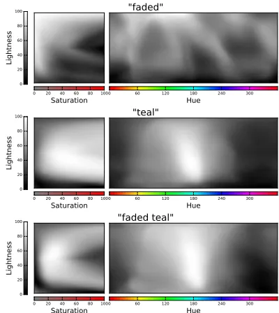
Compositionality Our model generalizes to com-positional descriptions not found in the training set. Fig. 3 visualizes the probability assigned to the
0 20 40 60 80 100 Li gh tn ess
0 20 40 60 80 100 Saturation
0 60 120 180 240 300
Hue "faded" 0 20 40 60 80 100 Li gh tn ess
0 20 40 60 80 100 Saturation
0 60 120 180 240 300
Hue "teal" 0 20 40 60 80 100 Li gh tn ess
0 20 40 60 80 100
Saturation 0 60 120 Hue180 240 300
"faded teal"
Figure 3:Conditional likelihood of “faded”, “teal”, and “faded teal”. The two meaning components can be seen in the two cross-sections: “faded” denotes a low saturation value, and “teal” denotes hues near the center of the spectrum.
0 20 40 60 80 100 Li gh tn ess
0 20 40 60 80 100 Saturation
0 60 120 180 240 300
Hue "greenish" 0 20 40 60 80 100 Li gh tn ess
0 20 40 60 80 100
Saturation 0 60 120 Hue180 240 300
[image:4.612.323.524.332.480.2]"greenish"
Figure 4:Conditional likelihood of “greenish” as a function of color. The distribution is bimodal, including greenish yellows and blues but not true greens. Top: LUX; bottom: our model.
novel utterance “faded teal”, along with “faded” and “teal” individually. The meaning of “faded teal” is intersective: “faded” colors are lower in saturation, excluding the colors of the rainbow (the V on the right side of the left panel); and “teal” denotes col-ors with a hue near 180° (center of the right panel).
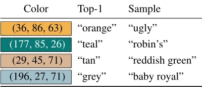
[image:4.612.94.277.369.429.2]Color Top-1 Sample (36, 86, 63) “orange” “ugly”
(177, 85, 26) “teal” “robin’s”
[image:5.612.83.287.59.147.2](29, 45, 71) “tan” “reddish green” (196, 27, 71) “grey” “baby royal”
Table 3:Error analysis: some color descriptions sampled from our model that are incorrect or incomplete.
“greenish” (Fig. 4) has such a denotation: “green-ish” specifies a region of color space surrounding, but not including, true greens.
Error analysis Table 3 shows some examples of errors found in samples taken from the model. The main type of error the system makes is ungrammati-cal descriptions, particularly fragments lacking a ba-sic color term (e.g., “robin’s”). Rarer are grammati-cal but meaningless compositions (“reddish green”) and false descriptions. When queried for its single most likely prediction,arg maxdS(d|c), the result
is nearly always an acceptable, “safe” description— manual inspection of 200 such top-1 predictions did not identify any errors.
5 Conclusion and future work
We presented a model for generating composi-tional color descriptions that is capable of produc-ing novel descriptions not seen in trainproduc-ing and sig-nificantly outperforms prior work at conditional lan-guage modeling.3 One natural extension is the use of character-level sequence modeling to capture complex morphology (e.g., “-ish” in “greenish”). Kawakami et al. (2016) build character-level mod-els for predicting colors given descriptions in addi-tion to describing colors. Their model uses a Lab-space color representation and uses the color to ini-tialize the LSTM instead of feeding it in at each time step; they also focus on visualizing point predictions of their description-to-color model, whereas we ex-amine the full distributions implied by our color-to-description model.
Another extension we plan to investigate is mod-eling of context, to capture how people describe col-ors differently to contrast them with other colcol-ors via
3We release our code at https://github.com/
stanfordnlp/color-describer.
pragmatic reasoning (DeVault and Stone, 2007; Gol-land et al., 2010; Monroe and Potts, 2015).
Acknowledgments
We thank Jiwei Li, Jian Zhang, Anusha Balakrish-nan, and Daniel Ritchie for valuable advice and discussions. This research was supported in part by the Stanford Data Science Initiative, NSF BCS 1456077, and NSF IIS 1159679.
References
Hirotugu Akaike. 1974. A new look at the statistical model identification. IEEE Transactions on Automatic
Control, 19(6):716–723.
Rami Al-Rfou, Guillaume Alain, Amjad Almahairi, Christof Angermueller, Dzmitry Bahdanau, Nicolas Ballas, et al. 2016. Theano: A Python framework for fast computation of mathematical expressions. arXiv
preprint arXiv:1605.02688.
Brent Berlin and Paul Kay. 1991. Basic color terms:
Their universality and evolution. University of
Cali-fornia Press.
David DeVault and Matthew Stone. 2007. Managing ambiguities across utterances in dialogue. In Ron Art-stein and Laure Vieu, editors,Proceedings of DECA-LOG 2007: Workshop on the Semantics and
Pragmat-ics of Dialogue.
Sander Dieleman, Jan Schlüter, Colin Raffel, Eben Ol-son, Søren Kaae Sønderby, Daniel Nouri, et al. 2015. Lasagne: First release.
John Duchi, Elad Hazan, and Yoram Singer. 2011. Adaptive subgradient methods for online learning and stochastic optimization. The Journal of Machine
Learning Research, 12:2121–2159.
Xavier Glorot and Yoshua Bengio. 2010. Understand-ing the difficulty of trainUnderstand-ing deep feedforward neural networks. InAISTATS.
Dave Golland, Percy Liang, and Dan Klein. 2010. A game-theoretic approach to generating spatial descrip-tions. InEMNLP.
Alex Graves. 2013. Generating sequences with recurrent neural networks. arXiv preprint arXiv:1308.0850. Geoffrey E. Hinton, Nitish Srivastava, Alex Krizhevsky,
Ilya Sutskever, and Ruslan R. Salakhutdinov. 2012. Improving neural networks by preventing co-adaptation of feature detectors. arXiv preprint
arXiv:1207.0580.
Kazuya Kawakami, Chris Dyer, Bryan Routledge, and Noah A. Smith. 2016. Character sequence models for colorful words. InEMNLP.
Emiel Krahmer and Kees Van Deemter. 2012. Compu-tational generation of referring expressions: A survey.
Computational Linguistics, 38(1):173–218.
Girish Kulkarni, Visruth Premraj, Sagnik Dhar, Siming Li, Yejin Choi, Alexander C. Berg, et al. 2011. Baby talk: Understanding and generating image descrip-tions. InCVPR.
Brian McMahan and Matthew Stone. 2015. A Bayesian model of grounded color semantics. Transactions of
the Association for Computational Linguistics, 3:103–
115.
Margaret Mitchell, Xufeng Han, Jesse Dodge, Alyssa Mensch, Amit Goyal, Alex Berg, et al. 2012. Midge: Generating image descriptions from computer vision detections. InEACL.
Will Monroe and Christopher Potts. 2015. Learning in the Rational Speech Acts model. InProceedings of the
20th Amsterdam Colloquium.
Randall Munroe. 2010. Color survey results. Online at http://blog.xkcd.com/2010/05/03/color-surveyresults. Sebastian Padó, 2006. User’s guide to sigf:
Significance testing by approximate
randomisa-tion. http://www.nlpado.de/~sebastian/
software/sigf.shtml.
Dengsheng Zhang and Guojun Lu. 2002. Shape-based image retrieval using generic Fourier descriptor.
Sig-nal Processing: Image Communication, 17(10):825–