A Joint Learning Model of Word Segmentation, Lexical Acquisition,
and Phonetic Variability
Micha Elsner [email protected]
Dept. of Linguistics The Ohio State University
Sharon Goldwater [email protected]
ILCC, School of Informatics University of Edinburgh
Naomi H. Feldman [email protected] Dept. of Linguistics University of Maryland
Frank Wood
[email protected] Dept. of Engineering University of Oxford
Abstract
We present a cognitive model of early lexi-cal acquisition which jointly performs word segmentation and learns an explicit model of phonetic variation. We define the model as a Bayesian noisy channel; we sample segmen-tations and word forms simultaneously from the posterior, using beam sampling to control the size of the search space. Compared to a pipelined approach in which segmentation is performed first, our model is qualitatively more similar to human learners. On data with vari-able pronunciations, the pipelined approach learns to treat syllables or morphemes as words. In contrast, our joint model, like infant learners, tends to learn multiword collocations. We also conduct analyses of the phonetic variations that the model learns to accept and its patterns of word recognition errors, and relate these to de-velopmental evidence.
1 Introduction
By the end of their first year, infants have acquired many of the basic elements of their native language. Their sensitivity to phonetic contrasts has become language-specific (Werker and Tees, 1984), and they have begun detecting words in fluent speech (Jusczyk and Aslin, 1995; Jusczyk et al., 1999) and learn-ing word meanlearn-ings (Bergelson and Swlearn-ingley, 2012). These developmental cooccurrences lead some re-searchers to propose that phonetic and word learning occur jointly, each one informing the other (Swingley, 2009; Feldman et al., 2013). Previous computational models capture some aspects of this joint learning
problem, but typically simplify the problem consid-erably, either by assuming an unrealistic degree of phonetic regularity for word segmentation (Goldwa-ter et al., 2009) or assuming pre-segmented input for phonetic and lexical acquisition (Feldman et al., 2009; Feldman et al., in press; Elsner et al., 2012). This paper presents, to our knowledge, the first broad-coverage model that learns to segment phonetically variable input into words, while simultaneously learn-ing an explicit model of phonetic variation that allows it to cluster together segmented tokens with different phonetic realizations (e.g.,[ju]and[jI]) into lexical items (/ju/).
We base our model on the Bayesian word segmen-tation model of Goldwater et al. (2009) (henceforth GGJ), using a noisy-channel setup where phonetic variation is introduced by a finite-state transducer (Neubig et al., 2010; Elsner et al., 2012). This in-tegrated model allows us to examine how solving the word segmentation problem should affect infants’ strategies for learning about phonetic variability and how phonetic learning can allow word segmentation to proceed in ways that mimic the idealized input used in previous models.
In particular, although the GGJ model achieves high segmentation accuracy on phonemic (non-variable) input and makes errors that are qualitatively similar to human learners (tending to undersegment the input), its accuracy drops considerably on phonet-ically noisy data and it tends to oversegment rather than undersegment. Here, we demonstrate that when the model is augmented to account for phonetic vari-ability, it is able to learn common phonetic changes
and by doing so, its accuracy improves and its errors return to the more human-like undersegmentation pattern. In addition, we find small improvements in lexicon accuracy over a pipeline model that seg-ments first and then performs lexical-phonetic learn-ing (Elsner et al., 2012). We analyze the model’s phonetic and lexical representations in detail, draw-ing comparisons to experimental results on adult and infant speech processing. Taken together, our results support the idea that a Bayesian model that jointly performs word segmentation and phonetic learning provides a plausible explanation for many aspects of early phonetic and word learning in infants.
2 Related Work
Nearly all computational models used to explore the problems addressed here have treated the learning tasks in isolation. Examples include models of word segmentation from phonemic input (Christiansen et al., 1998; Brent, 1999; Venkataraman, 2001; Swing-ley, 2005) or phonetic input (Fleck, 2008; Rytting, 2007; Daland and Pierrehumbert, 2011; Boruta et al., 2011), models of phonetic clustering (Vallabha et al., 2007; Varadarajan et al., 2008; Dupoux et al., 2011) and phonological rule learning (Peperkamp et al., 2006; Martin et al., 2013).
Elsner et al. (2012) present a model that is similar to ours, using a noisy channel model implemented with a finite-state transducer to learn about phonetic variability while clustering distinct tokens into lexi-cal items. However (like the earlier lexilexi-cal-phonetic learning model of Feldman et al. (2009; in press)) their model assumes known word boundaries, so to perform both segmentation and lexical-phonetic learning, they use a pipeline that first segments using GGJ and then applies their model to the results.
Neubig et al. (2010) also present a transducer-based noisy channel model that performs joint in-ference on two out of the three tasks we consider here; their model assumes fixed probabilities for pho-netic changes (the noise model) and jointly infers the word segmentation and lexical items, as in our ‘oracle’ model below (though unlike our system their model learns from phone lattices rather than a single transcription). They evaluate only on phone recogni-tion, not scoring the inferred lexical items.
Recently, B¨orschinger et al. (2013) did present a
α
Geom a, b, ..., ju, ... want, ... juwant, ...
Generator for possible words
Probabilities for each word (sparse)
p(ði) = .1, p(a) = .05, p(want) = .01...
∞ contexts
Conditional probabilities for each word after each word
p(ði | want) = .3, p(a | want) = .1, p(want | want) = .0001...
G
Gx
α
1n utterances
x1 x2 ...
Intended forms
ju want ə kuki ju want ɪt ...
s1 s2 ...
0 0
Surface forms
jə wan ə kuki ju wand ɪt ...
T
GGJ 09
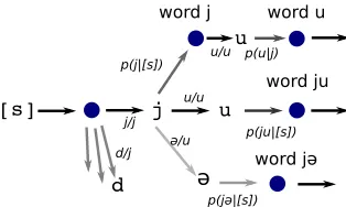
Figure 1: The graphical model for our system (Eq. 1-4). Note that thesi are not distinct observations; they are concatenated together into a continuous sequence of characters which constitute the observations.
joint learner for segmentation, phonetic learning, and lexical clustering, but the model and inference are tailored to investigate word-final /t/-deletion, rather than aiming for a broad coverage system as we do.
3 Model
We follow several previous models of lexical acquisi-tion in adopting a Bayesian noisy channel framework (Eq. 1-4; Fig. 1). The model has two components:
asourcedistributionP(X)over utterances without
phonetic variabilityX, i.e.,intended forms(Elsner et al., 2012) and achannelornoisedistributionT(S|X)
that translates them into the observed surface forms
S. The boundaries between surface forms are then deterministically removed so that the actual observa-tions are just the unsegmented string of characters in the surface forms.
G0|α0, pstop∼DP(α0, Geom(pstop)) (1)
Gx|G0, α1 ∼DP(α1, G0) (2)
Xi|Xi−1 ∼GXi−1 (3)
S|X;θ∼T(S|X;θ) (4)
The source model is an exact copy of GGJ1: to generate the intended-form word sequencesX, we
1We use their best reported parameter values: α 0 =
sample a random language model from a hierarchi-cal Dirichlet process (Teh et al., 2006) with char-acter strings as atoms. To do so, we first draw a unigram distribution G0 from a Dirichlet process prior whose base distribution generates intended form word strings by drawing each phone in turn until the stop character is drawn (with probabilitypstop). Then, for each possible context wordx, we draw a condi-tional distribution on words following that context
Gx = P(Xi = •|Xi−1 = x)using G0 as a prior. Finally, we sample word sequencesx1. . . xnfrom the bigram model.
The channel model is a finite transducer with pa-rametersθwhich independently rewrites single char-acters from the intended string into charchar-acters of the surface string. We use MAP point estimates of these parameters; single characters (withoutn-gram con-text) are used for computational efficiency. Also for efficiency, the transducer can insert characters into the surface string, but cannot delete characters from the intended string. As in several previous phonolog-ical models (Dreyer et al., 2008; Hayes and Wilson, 2008), the probabilities are learned using a feature-based log-linear model. For features, we use all the unigram features from Elsner et al. (2012), which check faithfulness to voicing, place and manner of articulation (for example, fork→g, active features
arefaith-manner,faith-place,output-gand
voiceless-to-voiced).
Below, we present two methods for learning the transducer parametersθ. Theoracletransducer is es-timated using the gold-standard word segmentations and intended forms for the dataset; it represents the best possible approximation under our model of the actual phonetics of the dataset. We can also estimate the transducer using theEMalgorithm. We first ini-tialize a simple transducer by putting small weights on the faithfulness features to encourage phonologi-cally plausible changes. With this initial model, we begin running the sampler used to learn word segmen-tations. After several hundred sampler iterations, we start re-estimating the transducer by maximum likeli-hood after each iteration. We regularize our estimates by adding 200 pseudocounts for the rewritex→x
during training (rather than regularizing the weights for particular features). We also showsegment only results for a model without the transducer component (i.e.,S =X); this recovers the GGJ baseline.
4 Inference
Inference for this model is complicated for two rea-sons. First, the hypothesis space is extremely large. Since we allow the input string to be probabilistically lengthened, we cannot be sure how long it is, nor which characters it contains. Second, our hypothe-ses about nearby characters are highly correlated due to lexical effects. When deciding how to interpret
[w@nt], if we posit that the intended vowel is/2/, the word is likely to be/w2n/ “one” and the next word begins with/t/; if instead we posit that the vowel is/O/, the word is probably/wOnt/ “want”. Thus, inference methods that change only one character at a time are unlikely to mix well. Since they cannot simultaneously change the vowel and resegment the
/t/, they must pass through a low-probability inter-mediate state to get from one state to the other, so will tend to get stuck in a bad local minimum. A Gibbs sampler which inserts or deletes a single seg-ment boundary in each step (Goldwater et al., 2009) suffers from this problem.
Mochihashi et al. (2009) describe an inference method with higher mobility: a block sampler for the GGJ model that samples from the posterior over analyses of a whole utterance at once. This method encodes the model as a large HMM, using dynamic programming to select an analysis. We encode our own model in the same way, constructing the HMM and composing it with the transducer (Mohri, 2004) to form a larger finite-state machine which is still amenable to forward-backward sampling.
4.1 Finite-state encoding
Following Mochihashi et al. (2009) and Neubig et al. (2010), we can write the original GGJ model
as a Hidden Semi-Markov model. States in the
HMM, written ST:[w][C], are labeled with the
previous wordwand the sequence of charactersC
which have so far been incorporated into the current word. To produce a word boundary, we transition from ST:[w][C] to ST:[C][]with probability
P(xi = C|xi−1 = w). We can also add the next charactersto the current word, transitioning from
ə word jə p(jə|[s])
d
j u
word ju
[s]
word j
u
word u
p(j|[s]) p(u|j)
p(ju|[s]) j/j
d/j ə/u u/u
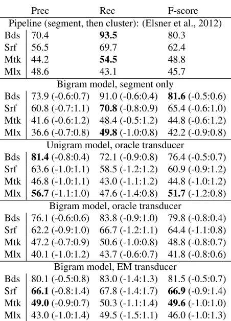
[image:4.612.107.264.56.150.2]u/u
Figure 2: A fragment of the composed finite-state machine for word segmentation and character replacement for the surface stringju. The start state [s] is followed by a word boundary (filled circle); the next intended character is probablyjbut can bedor others with lower probability. Afterj can be a word boundary (forming the intended wordj), or another character such asu,@or other (not shown) alternatives.
is no cost for the individual characters)2.
In addition to analyses using known words, we can also encode the uniform-geometric prior over unknown words using a finite-state machine. We can choose to select a word from the prior by tran-sitioning to a stateST:[Geom][]with probability
P(new word|xi−1 = w) immediately after a word boundary. While inGeom, we can transition to a new
Geomstate and produce any character with uniform probabilityP(c) = (1−Pstop)|C|1 ; otherwise, we can end the word, transitioning to ST:[unk.word][], with probabilityPstop.
This construction is also approximate; it ignores the possibility that the prior will generate a known wordw, in which case our final transition ought to be toST:[w][]instead ofST:[unk.word][]. This approximation means we do not need to add context to theGeomstate to remember the sequence of char-acters it produced, which allows us to keep only a singleGeomstate on the chart at each timestep.
When we compose this model with the channel model, the number of states expands. Each state must now keep track of the previous word, what intended charactersChave been posited and what surface
char-acters S have been recognized, ST:[w][C][S].
2
Though not mentioned by Mochihashi et al. (2009) or Neu-big et al. (2010), this construction is not exact, since transitions in a Bayesian HMM are exchangeable but not independent (Beal et al., 2001): if a word occurs twice in an utterance, its probabil-ity is slightly higher the second time. For single utterances, this bias is small and easy to correct for using a Metropolis-Hastings acceptance check (B¨orschinger and Johnson, 2012) using the path probability from the HMM as the proposal.
To recognize the current word, we transition to
ST:[C][][] with probabilityP(xi = C|xi−1 =
w). To parse a new surface charactersby positing intended character x (note thatx might be ), we transition toST:[w][C :x][S :s]with probabil-ityT(s|x). (As above, we pay no cost for our choice ofx, which is paid for when we recognize the word; however, we must pay fors.) For efficiency, we do not allow theG0states to hypothesize different sur-face and intended characters, so when we initially propose an unknown word, it must surface as itself.3
4.2 Beam sampler
This machine has too many states to fully fill the chart before backward sampling, so we restrict the set of trajectories under consideration using beam sampling (Van Gael et al., 2008) and simulated annealing.
The beam sampler is closely related to the standard beam search technique, which uses a probability cut-off to discard parts of the FST which are unlikely to figure in the eventual solution. Unlike conventional beam search, the sampler explores using stochastic cutoffs, so that all trajectories are explored, but most of the bad ones are explored infrequently, leading to higher efficiency.
We design our beam sampler to restrict the set of potential intended characters at each timestep. In particular, given a stream of input characters
S=s1. . . sn, we introduce a set of auxiliary cutoff variablesU =u1. . . un. Theuivariables represent limits on the probability of the emission of surface charactersi; we exclude any hypothesizedxiwhose probability of generating si, T(si|xi), is less than
ui. To create a beam sampling scheme, we must de-vise a distribution forU given a state sequenceQ(as discussed above, the sequence of states encodes the intended character sequence and the segmentation of the surface string),Pu(U|Q)and then incorporate the probability ofU into the forward messages.
Ifqiis the state inQat whichsiis generated, and
xithe corresponding intended character, we require that Pu < T(si|xi); that is, the cutoffs must not exclude any states in the sequenceQ. We definePu
as aλ-mixture of two distributions:
Pu(u|si, xi) =λU[0, min(.05, T(si|xi))]+
(1−λ)T(si|xi)Beta(5,1e−5)
The former distribution is quite unrestrictive, while the latter prefers to prune away nearly all the states. Thus, for most characters in the string, we do not permit radical changes, while for a fraction, we do.
We follow Huggins and Wood (2013), who ex-tended Van Gael et al. (2008) to the case of a non-uniformPu, to define our forward messageαas:
α(qi, i)∝P(qi, S0..i, U0..i) (5)
=X
qi−1
Pu(ui|si, xi)T(si|xi)α(qi−1, i−1)
This is the standard HMM forward message, aug-mented with the probability ofu. SincePu(·|si, xi) is required to be less thanT(si|xi), it will be 0 when-everT(si|xi)< u; this is how theuvariables func-tion as cutoffs. In practice, we use theuvariables to filter the lexical items that begin at each positioni
in advance, using a simple 0/1 edit distance Markov model which runs faster than our full model. (For ex-ample, we can quickly check if the currentU allows
wantas the intended form forwOlkati; if not, we can avoid constructing the prefixST:[xi−1][wa][wO] since the continuation will fail.)
The algorithm’s speed depends on the size and uncertainty of the inferred LM: large numbers of plausible words mean more states to explore. When inference starts, and the system is highly uncertain about word boundaries, it is therefore reasonable to limit the exploration of the character sequence. We do so by annealing in two ways: as in Goldwater et al. (2009), we raiseP(X) (Eq. 3) to a powert
which increases linearly from.3. To sample from the posterior, we would want to end witht= 1, but as in previous noisy-channel models (Elsner et al., 2012; Bahl et al., 1980) we get better results when we emphasize the LM at the expense of the channel and so end att= 2. Meanwhile, astrises and we explore fewer implausible lexical sequences, we can explore the character sequence more. We begin by setting theλinterpolation parameter ofPuto 0 to minimize exploration and increase it linearly to .3 (allowing the system to change about a third of the characters
on each sweep). This is similar to the scheme for alteringPuin Huggins and Wood (2013).
4.3 Dataset and metrics
We use the corpus released by Elsner et al. (2012), which contains 9790 child-directed English utter-ances originally from the Bernstein-Ratner corpus (Bernstein-Ratner, 1987) and later transcribed phone-mically (Brent, 1999). This standard word segmenta-tion dataset was modified by Elsner et al. (2012) to include phonetic variation by assigning each token a pronunciation independently selected from the empir-ical distribution of pronunciations of that word type in the closely-transcribed Buckeye Speech Corpus (Pitt et al., 2007). Following previous work, we hold out the last 1790 utterances as unseen test data during development. In the results presented here, we run the model on all 9790 utterances but score only these 1790. We average results over 5 runs of the model with different random seeds.
We use standard metrics for segmentation and lex-icon recovery. For segmentation, we report precision, recall and F-score for word boundaries (bds), and for the positions of word tokens in the surface string (srf; both boundaries must be correct).
For normalization of the pronunciation variation, we follow Elsner et al. (2012) in measuring how well the system clusters together variant pronunciations of the same lexical item, without insisting that the intended form the system proposes for them match the one in our corpus. For example, if the system correctly clusters[ju]and[jI] together but assigns them the incorrect intended form/jI/, we can still give credit to this cluster if it is the one that overlaps best with the gold-standard/ju/ cluster. To compute these scores, we find the optimal one-to-one map-ping between our clusters of pronunciations and the true lexical entries, then report scores for mapped to-kens (mtk; boundaries and mapping to gold standard cluster must be correct) and mapped types4(mlx).
4
Prec Rec F-score Pipeline (segment, then cluster): (Elsner et al., 2012)
Bds 70.4 93.5 80.3
Srf 56.5 69.7 62.4
Mtk 44.2 54.5 48.8
Mlx 48.6 43.1 45.7
Bigram model, segment only
Bds 73.9 (-0.6:0.7) 91.0 (-0.6:0.4) 81.6(-0.5:0.6) Srf 60.8 (-0.7:1.1) 70.8(-0.8:0.9) 65.4 (-0.6:1.0) Mtk 41.6 (-0.6:1.2) 48.4 (-0.5:1.2) 44.8 (-0.6:1.2) Mlx 36.6 (-0.7:0.8) 49.8(-1.0:0.8) 42.2 (-0.9:0.8)
Unigram model, oracle transducer
Bds 81.4(-0.8:0.4) 72.1 (-0.9:0.8) 76.4 (-0.5:0.7) Srf 63.6 (-1.0:1.1) 58.5 (-1.2:1.2) 60.9 (-0.9:1.2) Mtk 46.8 (-1.0:1.1) 43.0 (-1.1:1.2) 44.8 (-1.0:1.2) Mlx 56.7(-1.1:1.0) 47.6 (-1.4:0.8) 51.7(-1.2:0.8)
Bigram model, oracle transducer
Bds 76.1 (-0.6:0.6) 83.8 (-0.9:1.0) 79.8 (-0.8:0.4) Srf 62.2 (-0.9:1.0) 66.7 (-1.2:1.1) 64.4 (-1.1:0.8) Mtk 47.2 (-0.7:0.9) 50.6 (-1.0:0.8) 48.8 (-0.8:0.7) Mlx 40.1 (-1.0:1.2) 43.7 (-0.6:0.7) 41.8 (-0.8:0.6)
Bigram model, EM transducer
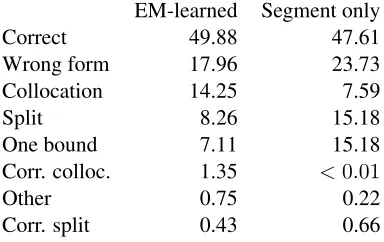
[image:6.612.75.301.53.367.2]Bds 80.1 (-0.5:0.8) 83.0 (-1.4:1.3) 81.5 (-0.5:0.7) Srf 66.1(-0.8:1.4) 67.8 (-1.4:1.7) 66.9(-0.9:1.4) Mtk 49.0(-0.9:0.7) 50.3 (-1.1:1.4) 49.6(-1.0:1.0) Mlx 43.0 (-1.0:1.4) 49.5 (-1.5:1.1) 46.0 (-1.0:1.3)
Table 1: Mean segmentation (bds,srf) and normalization (mtk,mlx) scores on the test set over 5 runs. Parentheses show min and max scores as differences from the mean.
5 Results and discussion
In the following sections, we analyze how our model with variability compares to GGJ on noisy data. We give quantitative scores and also show that qualitative patterns of errors are often similar to those of human learners and listeners.
5.1 Clean versus variable input
We begin by evaluating our model as a word seg-mentation system. (Table 1 gives segseg-mentation and normalization scores for various models and base-lines on the 1790 test utterances.) We first confirm that our inference method is reasonable. The bigram model without variability (“segment only”) should have the same segmentation performance as the stan-darddpsegimplementation of GGJ. This is the case:
dpseghas boundaryF of 80.3 and tokenF of 62.4; we get 81.6 and 65.4. Thus, our sampler is finding good solutions, at least for the no-variability model. We compare segmentation scores between the
“segment only” system and the two bigram models with transducers (“oracle” and “EM”). While these systems all achieve similar segmentation scores, they do so in different ways. “Segment only” finds a so-lution with boundary precision 73.9% and boundary recall 91.0% for a totalF of 81.6%. The low pre-cision and high recall here indicate a tendency to oversegment; when the analysis of a given subse-quence is unclear, the system prefers to chop it into small chunks. The bigram models which incorporate transducers scoreP: 76.1,R: 83.8 (oracle) andP: 80.1,R: 83.0 (EM), indicating that they prefer to find longer sequences (undersegment) more.
In previous experiments on datasets without varia-tion, GGJ also has a strong tendency to undersegment the data (boundaryP: 90.1,R: 80.3), which Gold-water et al. argue is rational behavior for an ideal learner seeking a parsimonious explanation for the data. Undersegmentation occurs especially when ig-noring lexical context (a unigram model), but to some extent even in bigram models. Human learners also tend to learn collocations as single words (Peters, 1983; Tomasello, 2000), and the GGJ model has been
shown to capture several other effects seen in labora-tory segmentation tasks (Frank et al., 2010). Together, these findings support the idea that human learners may behave in important respects like the Bayesian ideal learners that Goldwater et al. presented.
However, experiments on data with variation have called these conclusions into question. In particu-lar, GGJ has previously been shown to oversegment rather than undersegment as the input grows noisier (Fleck, 2008), and our results replicate this finding (oversegmentation for the “segment only” model). In addition, the GGJ bigram model, which achieves much higher segmentation accuracy than the unigram model on clean data, actually performs worse on very noisy data (Jansen et al., 2013). Infants are known to track statistical dependencies across words (G´omez and Maye, 2005), so it is worrisome that these de-pendencies hurt GGJ’s segmentation accuracy when learning from noisy data.
un-dersegmentation. Thus, their qualitative performance on variable data resembles GGJ’s on clean data, and therefore the behavior of human learners.
5.2 Phonetic variability
We next analyze the model’s ability to normalize vari-ations in the pronunciation of tokens, by inspecting themtkscore. The “segment only” baseline is pre-dictably poor,F: 44.8. The pipeline model scores 48.8, and our oracle transducer model matches this exactly. The EM transducer scores better,F: 49.6. Although the confidence intervals overlap slightly, the EM system also outperforms the pipeline on the otherF-measures; altogether, these results suggest at least a weak learning synergy (Johnson, 2008) be-tween segmentation and phonetic learning.
It is interesting that EM can perform better than the oracle. However, EM is more conservative about which sound changes it will allow, and thus tends to avoid mistakes caused by the simplicity of the trans-ducer model. Since the transtrans-ducer works segment-by-segment, it can apply rare contextual variations out of context. EM benefits from not learning these variations to begin with.
We can also compare the bigram and unigram ver-sions of the model. The unigram model is a rea-sonable segmenter, though not quite as good as the bigram model, with boundaryF of 76.4 and token
F of 60.9 (compared to 79.8 and 64.4 using the bi-gram model). However, it is not good at normalizing variation; itsmtkscore is comparable to the baseline at 44.8%5. Although bigram context is only moder-ately effective for telling where words are, the model seems heavily reliant on lexical context to decide whatwords it is hearing.
5.3 Error analysis
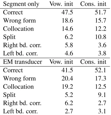
To gain more insight into the differing behavior of our model versus a pipelined system, we inspect the intended word stringsX proposed by each one in detail. Below, we categorize the kinds of intended word strings that the model might propose to span a given gold-standard word token:
Correct Correctly segmented, mapped to the correct lexical item (e.g., gold intended/ju/, surface
5Elsner et al. (2012) show a similar result for a unigram version of their pipelined system.
EM-learned Segment only
Correct 49.88 47.61
Wrong form 17.96 23.73
Collocation 14.25 7.59
Split 8.26 15.18
One bound 7.11 15.18
Corr. colloc. 1.35 <0.01
Other 0.75 0.22
[image:7.612.318.510.59.180.2]Corr. split 0.43 0.66
Table 2: Distribution (%) of error types (see text) in a single run on the full dataset.
segmentation[ju], intended/ju/)
Wrong form Correctly segmented, mapped to the wrong lexical item (/ju/, surf. [ju], int. /jEs/) Colloc Missegmented as part of a sequence whose
boundaries correspond to real word boundaries (/ju•want/, surf.[juwant], int./juwant/) Corr. colloc As above, but proposed lexical item
maps to this word (/ar•ju/, surf. [arj@] int.
/ju/)
Split Missegmented with a word-internal boundary (/dOgiz/, surf. [dO•giz], int./dO•giz/)
Corr. split As above, but one proposed word maps correctly (/dOgi/, surf. [dOg•i], int./dOgi•@/) One boundary One boundary correct, the other
wrong (/ju•wa. . . /, surf.[juw], int./juw/) Other Not a collocation, both boundaries are wrong
(/du•ju•wa. . . /, surf.[ujuw], int./ujuw/)
EM ju: 805,duju: 239,juwan: 88,jI: 58,e~ju: 54,judu: 47,jæ: 39,jul2k: 39,Su: 30,u: 23,Zu: 18,j: 17,
je~: 16,tSu: 15,aj:15,Derjugo: 12,dZu: 12
GGJ ju: 498,jI: 280,j@: 165,ji: 119,duju: 106,dujI: 44,
kInju: 39,i: 32,u: 29,kInjI: 29,jul2k: 24,juwan: 23,j: 22,Su: 19,jU: 18,e~ju: 18,I:16,Zu: 15,dZ•u: 13,jE: 12,SI: 11,TæNkju: 11
Table 3: Forms proposed with frequency > 10 for gold-standard tokens of “you” in one sample from EM-transducer and segment-only (GGJ) system.
To illustrate this behavior anecdotally, we present the distribution of intended word strings spanning tokens whose gold intended form is/ju/ “you” (Table 3). The EM-learned solution proposes 805 tokens of/ju/, which is the correct analysis6; the “segment only” system instead finds varying forms like/jI/,
/jæ/etc. This is unsurprising and could be repaired by a suitable pipelined system. However, the EM system also proposes 239 instances of “doyou”, 88 instances of “youwant”, 54 instances of “areyou” and several other collocations. The “segment only” sys-tem finds some of these collocations, split into dif-ferent versions: for instance 106 instances of/duju/
and 44 of/dujI/. In a pipelined system, we could combine these variants to find 150 instances— but this is still 89 instances short of the 239 found when allowing for variability. The same pattern holds for “youlike” and “youwant”. Because the non-variable system must learn each variant separately, it learns only the most common instances of these long collo-cations, and analyzes infrequent variants differently. We also perform this analysis specifically for words beginning with vowels. Infants show a delay in their ability to segment these words from continu-ous speech (Mattys and Jusczyk, 2001; Nazzi et al., 2005; Seidl and Johnson, 2008), and Seidl and John-son (2008) suggest a perceptual explanation— initial vowels can be hard to hear and often exhibit variation due to coarticulation or resyllabification. Although our dataset does not contain coarticulation as such, it should show this pattern of greater variation, which we hypothesize might lead to difficulty in segmenting and recognizing vowel-initial words.
The model’s behavior is consistent with this hy-pothesis (Table 4). Both the “segment only” and EM transducer models find approximately the same
6Not all the variants are merged, however.jI,jæ,Suetc. are still occasionally analyzed as separate lexical items.
Segment only Vow. init Cons. init
Correct 47.5 51.7
Wrong form 18.6 15.7
Collocation 14.6 12.2
Split 6.2 10.8
Right bd. corr. 5.8 3.6
Left bd. corr. 4.6 3.8
EM transducer Vow. init Cons. init
Correct 41.5 52.1
Wrong form 20.4 17.3
Collocation 19.2 12.5
Split 5.2 9.1
Right bd. corr. 6.2 2.7
[image:8.612.314.496.58.246.2]Left bd. corr. 2.7 3.1
Table 4: Most common error types (%; see text) for in-tended forms beginning with vowels or consonants. Rare error types are not shown. “One bound” errors are split up by which boundary is correct.
proportion of vowel-initial tokens, and both systems do somewhat better on consonant-initial words than vowel-initial words. The advantage is stronger for the transducer model, which gets only 41.5% of vowel-initial tokens correct as opposed to 52.1% of consonant-initial words. It proposes more colloca-tions for vowel-initial words (19.2%) than for conso-nants (12.5%). In cases where they do not propose a collocation, both systems are somewhat more likely to find the right boundary of a vowel-initial token than the left boundary (although again this difference is larger for the EM system); this suggests that the problem is indeed caused by the initial segment.
5.4 Phonetic Learning
abil-ity to generalize across talkers, affects, and dialects. They have difficulty recognizing word tokens that are spoken by a different talker or in a different tone of voice until 11 months (Houston and Jusczyk, 2000; Singh et al., 2004), and the ability to adapt to unfa-miliar dialects appears to develop even later, between 15 and 19 months (Best et al., 2009; Heugten and Johnson, in press; White and Aslin, 2011).
Similar to infants, our model shows both a vowel-consonant asymmetry and a reluctance to accept the full range of adult phonetic variability. Table 5 shows some segment-to-segment alternations learned in var-ious transducers. The oracle learns a large amount of variation (u surfaces as itself only 68% of the time) involving many different segments, whereas EM is similar to infant learners in learning a more conservative solution with fewer alternations over-all. Moreover, EM appears to identify patterns of variability in vowels before consonants. It learns a similar range of alternations foru as in the oracle, although it treats the sound as less variable than it actually is. It learns much less variability for con-sonants; it picks up the alternation ofD withsand
z, but predicts thatD will surface as itself 91% of the time when the true figure is only 69%. And it fails to learn any meaningful alternations involving
k. These results suggest that patterns of variability in vowels are more evident than patterns of variability in consonants when infants are beginning to solve the word segmentation problem.
To investigate the effect of data size on this con-servativism, we ran the system on 1000 utterances instead of 9790. This leads to an even more conser-vative solution, with variations forubut none of the others (althoughiandD still vary more thank).
5.5 Segmentation and recognition errors
A particularly interesting set of errors are those that involve both a missegmentation and a simultaneous misrecognition, since the joint model is prone to such errors while the pipelined model is not. Rel-atively little is known about infants’ misrecognitions of words in fluent speech, although it is clear that they find words in medial position harder (Plunkett, 2005; Seidl and Johnson, 2006). However, adults make missegmentation/misrecognition errors fairly often, especially when listening to noisy audio (Butterfield and Cutler, 1988). Such errors are more common
System x top 4 outputss
Oracle
u u .68 @ .05 a .04 U .04
i i .85 I .03 @ .03 E .02
D D .69 s .07 [φ] .07 z .04
k k .93 d .02 g .02
[φ] r .21 h .11 d .01 @ .07
EM (full)
u u .75 @ .08 I .04 U .03
i i .90 I .04 E .02
D D .91 s .03 z 0.1
k k .98
[φ] @ .32 I .14 n .13 t .13
EM (only 1000
utts)
u u .82 I .04 @ .04 a .02
i i .97
D D .95
k k .99
[image:9.612.314.523.57.272.2][φ] @ .21 I .18 t .12 s .12
Table 5: Learned phonetic alternations: top 4 outputss
withp > .001for inputsx=uw (/u/), iy (/i/), dh (/D/), k (/k/) and [φ], the null character. Outputs from [φ] are insertions. The oracle allows [φ] as an output (deletion) but for computational reasons, the model does not.
when the misrecognized word belongs to a prosod-ically rare class and when the incorrectly hypothe-sized string contains frequent words (Cutler, 1990); phonetically ambiguous words are also more com-monly recognized as the more frequent of two op-tions (Connine et al., 1993). For the indefinite article “a” (often reduced to[@]), lexical context is the main factor in deciding between ambiguous interpretations (Kim et al., 2012). In rapid speech, listeners have few phonetic cues to indicate whether it is present at all (Dilley and Pitt, 2010). Below, we analyze various misrecognitions made by our system (using the EM transducer), and find some similar effects.
The easiest cases to analyze are those with no mis-segmentation: the proposed boundaries are correct, and the proposed lexical entry corresponds to a real word7, but not the correct one. Most of them corre-spond to homophones (Table 6).
Common cases with a missegmentation includeit
andis,aandis,it’sandis,who,who’sandwhose,
that’sandwhat’s, andthereandthere’s. In general,
these errors involve words which sometimes appear
7
Actual proposed count
/tu/“two” /t@/“to” 95
/kin/ “can” /kænt/“can’t” 67
/En/ “and” /æn/“an” 61
/hIz/ “his” /Iz/“is” 57
/D@/ “the” /@/“ah” 51
/w@ts/ “what’s” /wants/“wants” 40
/wan/“want” /won/“won’t” 39
/yu/ “you” /yæ/“yeah” 39
/f@~/ “for” /fOr/“four” 30
[image:10.612.77.262.58.187.2]/hir/“here” /hil/“he’ll” 28
Table 6: Top ten errors involving confusion between real, correctly segmented words: the most common pronunci-ation of the actual token and its orthographic form, the same for the proposed token, and the frequency.
with a morpheme or clitic (which can easily be mis-segmented as part of something else), words which differ by one segment, and frequent function words which often appear in similar contexts. These tenden-cies match those shown by adult human listeners.
A particularly distinctive set of joint recognition and segmentation errors are those where an entire real token is treated as phonetic “noise”— that is, it is segmented along with an adjacent word, and the system clusters the whole sequence as a token of that word. The most common examples are “that’s a” identified as “that’s”, “have a” identified as “have”, “sees a” identified as “sees” and other examples in-volving “a”, a word which also frequently confuses humans (Kim et al., 2012; Dilley and Pitt, 2010). However, there are also instances of “who’s in” as “who’s”, “does it” as “does”, and “can you” as “can”.
6 Conclusion
We have presented a model that jointly infers word segmentation, lexical items, and a model of phonetic variability; we believe this is the first model to do so on a broad-coverage naturalistic corpus8. Our re-sults show a small improvement in both segmentation and normalization over a pipeline model, providing evidence for a synergistic interaction between these learning tasks and supporting claims of interactive learning from the developmental literature on infants. We also reproduced several experimental findings; our results suggest that two vowel-consonant
asym-8
Software is available from the ACL archive; updated versions may be posted at https://bitbucket.org/ melsner/beamseg.
metries, one from the word segmentation literature and another from the phonetic learning literature, are linked to the large variability in vowels found in nat-ural corpora. The model’s correspondence with hu-man behavioral results is by no means exact, but we believe these kinds of predictions might help guide future research on infant phonetic and word learning.
Acknowledgements
Thanks to Mary Beckman for comments. This work was supported by EPSRC grant EP/H050442/1 to the second author.
References
Lalit Bahl, Raimo Bakis, Frederick Jelinek, and Robert Mercer. 1980. Language-model/acoustic-channel-model balance mechanism. Technical disclosure bul-letin Vol. 23, No. 7b, IBM, December.
Matthew J. Beal, Zoubin Ghahramani, and Carl Edward Rasmussen. 2001. The infinite Hidden Markov Model. InNIPS, pages 577–584.
Elika Bergelson and Daniel Swingley. 2012. At 6-9 months, human infants know the meanings of many common nouns.Proceedings of the National Academy of Sciences, 109:3253–3258.
Nan Bernstein-Ratner. 1987. The phonology of parent-child speech. In K. Nelson and A. van Kleeck, editors, Children’s Language, volume 6. Erlbaum, Hillsdale, NJ.
Catherine T. Best, Michael D. Tyler, Tiffany N. Good-ing, Corey B. Orlando, and Chelsea A. Quann. 2009. Development of phonological constancy: Toddlers’ per-ception of native- and jamaican-accented words. Psy-chological Science, 20(5):539–542.
Benjamin B¨orschinger and Mark Johnson. 2012. Using rejuvenation to improve particle filtering for Bayesian word segmentation. InProceedings of the 50th Annual Meeting of the Association for Computational Linguis-tics (Volume 2: Short Papers), pages 85–89, Jeju Island, Korea, July. Association for Computational Linguistics. Benjamin B¨orschinger, Mark Johnson, and Katherine De-muth. 2013. A joint model of word segmentation and phonological variation for English word-final /t/-deletion. InProceedings of the 51st Annual Meeting of the Association for Computational Linguistics, Sofia, Bulgaria, August. Association for Computational Lin-guistics.
phonetic variation. InProceedings of the 2nd Workshop on Cognitive Modeling and Computational Linguistics, pages 1–9.
Laura Bosch and N´uria Sebasti´an-Gall´es. 2003. Simulta-neous bilingualism and the perception of a language-specific vowel contrast in the first year of life. Lan-guage and Speech, 46(2-3):217–243.
Michael R. Brent. 1999. An efficient, probabilistically sound algorithm for segmentation and word discovery. Machine Learning, 34:71–105, February.
Sally Butterfield and Anne Cutler. 1988. Segmentation errors by human listeners: Evidence for a prosodic segmentation strategy. InProceedings of SPEECH ‘88: Seventh Symposium of the Federation of Acoustic Societies of Europe, vol. 3, pages 827–833, Edinburgh. Morten H. Christiansen, Joseph Allen, and Mark S. Sei-denberg. 1998. Learning to Segment Speech Using Multiple Cues: A Connectionist Model.Language and Cognitive Processes, 13(2/3):221–269.
C. M. Connine, D. Titone, and J. Wang. 1993. Audi-tory word recognition: Extrinsic and intrinsic effects of word frequency. Journal of Experimental Psychology: Learning, Memory and Cognition, 19:81–94.
Anne Cutler. 1990. Exploiting prosodic probabilities in speech segmentation. In G. A. Altmann, editor, Cog-nitive models of speech processing: Psycholinguistic and computational perspectives, pages 105–121. MIT Press, Cambridge, MA.
Robert Daland and Janet B. Pierrehumbert. 2011. Learn-ing diphone-based segmentation. Cognitive Science, 35(1):119–155.
Laura C. Dilley and Mark Pitt. 2010. Altering context speech rate can cause words to appear or disappear. Psychological Science, 21(11):1664–1670.
Markus Dreyer, Jason R. Smith, and Jason Eisner. 2008. Latent-variable modeling of string transductions with finite-state methods. InProceedings of the Conference on Empirical Methods in Natural Language Processing, EMNLP ’08, pages 1080–1089, Stroudsburg, PA, USA. Association for Computational Linguistics.
Emmanuel Dupoux, Guillaume Beraud-Sudreau, and Shigeki Sagayama. 2011. Templatic features for mod-eling phoneme acquisition. InProceedings of the 33rd Annual Cognitive Science Society.
Micha Elsner, Sharon Goldwater, and Jacob Eisenstein. 2012. Bootstrapping a unified model of lexical and pho-netic acquisition. InProceedings of the 50th Annual Meeting of the Association for Computational Linguis-tics (Volume 1: Long Papers), pages 184–193, Jeju Island, Korea, July. Association for Computational Lin-guistics.
Naomi Feldman, Thomas Griffiths, and James Morgan. 2009. Learning phonetic categories by learning a
lexi-con. InProceedings of the 31st Annual Conference of the Cognitive Science Society.
Naomi H. Feldman, Emily B. Myers, Katherine S. White, Thomas L. Griffiths, and James L. Morgan. 2013. Word-level information influences phonetic learning in adults and infants.Cognition, 127(3):427–438. Naomi H. Feldman, Thomas L. Griffiths, Sharon
Gold-water, and James L. Morgan. in press. A role for the developing lexicon in phonetic category acquisition. Psychological Review.
Margaret M. Fleck. 2008. Lexicalized phonotactic word segmentation. InProceedings of ACL-08: HLT, pages 130–138, Columbus, Ohio, June. Association for Com-putational Linguistics.
Michael C. Frank, Sharon Goldwater, Thomas L. Griffiths, and Joshua B. Tenenbaum. 2010. Modeling human per-formance in statistical word segmentation.Cognition, 117(2):107–125.
Sharon Goldwater, Thomas L. Griffiths, and Mark John-son. 2009. A Bayesian framework for word segmen-tation: Exploring the effects of context. Cognition, 112(1):21–54.
Rebecca G´omez and Jessica Maye. 2005. The develop-mental trajectory of nonadjacent dependency learning. Infancy, 7:183–206.
Bruce Hayes and Colin Wilson. 2008. A maximum en-tropy model of phonotactics and phonotactic learning. Linguistic Inquiry, 39(3):379–440.
Marieke van Heugten and Elizabeth K. Johnson. in press. Learning to contend with accents in infancy: Benefits of brief speaker exposure. Journal of Experimental Psychology: General.
Derek M. Houston and Peter W. Jusczyk. 2000. The role of talker-specific information in word segmentation by infants.Journal of Experimental Psychology: Human Perception and Performance, 26:1570–1582.
Jonathan Huggins and Frank Wood. 2013. Infinite struc-tured hidden semi-Markov models. Transactions on Pattern Analysis and Machine Intelligence (TPAMI), to appear, September.
Mark Johnson. 2008. Using adaptor grammars to identify synergies in the unsupervised acquisition of linguis-tic structure. InProceedings of ACL-08: HLT, pages 398–406, Columbus, Ohio, June. Association for Com-putational Linguistics.
Peter W. Jusczyk and Richard N. Aslin. 1995. Infants’ de-tection of the sound patterns of words in fluent speech. Cognitive Psychology, 29:1–23.
Peter W. Jusczyk, Derek M. Houston, and Mary Newsome. 1999. The beginnings of word segmentation in English-learning infants.Cognitive Psychology, 39:159–207. Dahee Kim, Joseph D.W. Stephens, and Mark A. Pitt.
2012. How does context play a part in splitting words apart? Production and perception of word boundaries in casual speech. Journal of Memory and Language, 66(4):509 – 529.
Patricia K. Kuhl, Karen A. Williams, Francisco Lacerda, Kenneth N. Stevens, and Bjorn Lindblom. 1992. Lin-guistic experience alters phonetic perception in infants by 6 months of age.Science, 255(5044):606–608. Leigh Lisker and Arthur S. Abramson. 1964. A
cross-language study of voicing in initial stops: Acoustical measurements.Word, 20:384–422.
Andrew Martin, Sharon Peperkamp, and Emmanuel Dupoux. 2013. Learning phonemes with a proto-lexicon.Cognitive Science, 37:103–124.
Sven L. Mattys and Peter W. Jusczyk. 2001. Do infants segment words or recurring contiguous patterns? Jour-nal of Experimental Psychology: Human Perception and Performance, 27(3):644–655+.
Jessica Maye, Janet F. Werker, and LouAnn Gerken. 2002. Infant sensitivity to distributional information can affect phonetic discrimination.Cognition, 82(3):B101–11. Daichi Mochihashi, Takeshi Yamada, and Naonori Ueda.
2009. Bayesian unsupervised word segmentation with nested pitman-yor language modeling. InProceedings of the Joint Conference of the 47th Annual Meeting of the ACL and the 4th International Joint Conference on Natural Language Processing of the AFNLP, pages 100–108, Suntec, Singapore, August. Association for Computational Linguistics.
Mehryar Mohri, 2004.Weighted Finite-State Transducer Algorithms: An Overview, chapter 29, pages 551–564. Physica-Verlag.
Thierry Nazzi, Laura C. Dilley, Ann Marie Jusczyk, Ste-fanie Shattuck-Hufnagel, and Peter W. Jusczyk. 2005. English-learning infants’ segmentation of verbs from fluent speech.Language and Speech, 48(3):279–298+. Graham Neubig, Masato Mimura, Shinsuke Mori, and Tatsuya Kawahara. 2010. Learning a language model from continuous speech. In11th Annual Conference of the International Speech Communication Associa-tion (InterSpeech 2010), pages 1053–1056, Makuhari, Japan, 9.
Sharon Peperkamp, Rozenn Le Calvez, Jean-Pierre Nadal, and Emmanuel Dupoux. 2006. The acquisition of allophonic rules: Statistical learning with linguistic constraints.Cognition, 101(3):B31–B41.
Ann M. Peters. 1983. The Units of Language Acquisi-tion. Cambridge Monographs and Texts in Applied Psycholinguistics. Cambridge University Press. Gordon E. Peterson and Harold L. Barney. 1952. Control
methods used in a study of the vowels.Journal of the Acoustical Society of America, 24(2):175–184. Mark A. Pitt, Laura Dilley, Keith Johnson, Scott
Kies-ling, William Raymond, Elizabeth Hume, and Eric Fosler-Lussier. 2007. Buckeye corpus of conversa-tional speech (2nd release).
Kim Plunkett. 2005. Learning how to be flexible with words.Attention and Performance, XXI:233–248. Anton Rytting. 2007. Preserving Subsegmental
Varia-tion in Modeling Word SegmentaVaria-tion (Or, the Raising of Baby Mondegreen). Ph.D. thesis, The Ohio State University.
Amanda Seidl and Elizabeth Johnson. 2006. Infant word segmentation revisited: Edge alignment facilitates tar-get extraction. Developmental Science, 9:565–573. Amanda Seidl and Elizabeth Johnson. 2008. Perceptual
factors influence infants’ extraction of onsetless words from continuous speech. Journal of Child Language, 34.
Leher Singh, James Morgan, and Katherine White. 2004. Preference and processing: The role of speech affect in early spoken word recognition.Journal of Memory and Language, 51:173–189.
Daniel Swingley. 2005. Statistical clustering and the con-tents of the infant vocabulary. Cognitive Psychology, 50:86–132.
Daniel Swingley. 2009. Contributions of infant word learning to language development. Philosophical Transactions of the Royal Society B: Biological Sci-ences, 364(1536):3617–3632, December.
Y. W. Teh, M. I. Jordan, M. J. Beal, and D. M. Blei. 2006. Hierarchical Dirichlet processes. Journal of the Ameri-can Statistical Association, 101(476):1566–1581. Michael Tomasello. 2000. The item-based nature of
chil-dren’s early syntactic development.Trends in Cognitive Sciences, 4(4):156 – 163.
Gautam K. Vallabha, James L. McClelland, Ferran Pons, Janet F. Werker, and Shigeaki Amano. 2007. Unsuper-vised learning of vowel categories from infant-directed speech. Proceedings of the National Academy of Sci-ences, 104(33):13273–13278.
ICML ’08, pages 1088–1095, New York, NY, USA. ACM.
Balakrishnan Varadarajan, Sanjeev Khudanpur, and Em-manuel Dupoux. 2008. Unsupervised learning of acoustic sub-word units. In Proceedings of the As-sociation for Computational Linguistics: Short Papers, pages 165–168.
Anand Venkataraman. 2001. A statistical model for word discovery in transcribed speech. Computational Lin-guistics, 27(3):351–372.
Janet F. Werker and Richard C. Tees. 1984. Cross-language speech perception: Evidence for perceptual reorganization during the first year of life. Infant Be-havior and Development, 7(1):49 – 63.
![Table 5: Learned phonetic alternations: top 4 outputs swith p >. 001 for inputs x=uw (/u/), iy (/i/), dh (/D/),k (/k/) and [φ ], the null character](https://thumb-us.123doks.com/thumbv2/123dok_us/1367173.669853/9.612.314.523.57.272/table-learned-phonetic-alternations-outputs-swith-inputs-character.webp)
