Decoding with Finite-State Transducers on GPUs
Arturo Argueta and David Chiang
Department of Computer Science and Engineering University of Notre Dame
aargueta,[email protected]
Abstract
Weighted finite automata and transduc-ers (including hidden Markov models and conditional random fields) are widely used in natural language processing (NLP) to perform tasks such as morphological anal-ysis, part-of-speech tagging, chunking, named entity recognition, speech recog-nition, and others. Parallelizing finite state algorithms on graphics processing units (GPUs) would benefit many areas of NLP. Although researchers have imple-mented GPU versions of basic graph al-gorithms, limited previous work, to our knowledge, has been done on GPU algo-rithms for weighted finite automata. We introduce a GPU implementation of the Viterbi and forward-backward algorithm, achieving decoding speedups of up to 5.2x over our serial implementation running on different computer architectures and 6093x over OpenFST.
1 Introduction
Weighted finite automata (Mohri, 2009), includ-ing hidden Markov models and conditional ran-dom fields (Lafferty et al., 2001), are used to solve a wide range of natural language processing (NLP) problems, including phonology and morphology, part-of-speech tagging, chunking, named entity recognition, and others. Even models for speech recognition and phrase-based translation can be thought of as extensions of finite automata (Mohri et al., 2002; Kumar et al., 2005).
Although the use of graphics processing units (GPUs) is now de rigeur in applications of neu-ral networks and made easy through toolkits like Theano (Theano Development Team, 2016), there has been little previous work, to our knowledge,
on acceleration of weighted finite-state compu-tations on GPUs (Narasiman et al., 2011; Li et al., 2014; Peng et al., 2016; Chong et al., 2009). In this paper, we consider the operations that are most likely to have high speed require-ments: decoding using the Viterbi algorithm, and training using the forward-backward algorithm. We present an implementation of the Viterbi and forward-backward algorithms for CUDA GPUs. We release it as open-source software, with the hope of expanding in the future to a toolkit includ-ing other operations like composition.
Most previous work on parallel processing of finite automata (Ladner and Fischer, 1980; Hillis and Steele, 1986; Mytkowicz et al., 2014) uses dense representations of finite automata, which is only appropriate if the automata are not too sparse (that is, most states can transition to most other states). But the automata used for natural language tend to be extremely large and sparse. In addition, the more recent work in this line assumes deter-ministic automata, but automata that model natural language ambiguity are generally nondeterminis-tic.
Previous work has been done on accelerating particular NLP tasks on GPUs: in machine trans-lation, phrase-pair retrieval (He et al., 2013) and language model querying (Bogoychev and Lopez, 2016); parsing (Hall et al., 2014; Canny et al., 2013); and speech recognition (Kim et al., 2012). Our aim here is for a more general-purpose collec-tion of algorithms for finite automata.
Our work uses concepts from the work of Mer-rill et al. (2012), who show that GPUs can be used to accelerate breadth-first search in sparse graphs. Our approach is simple, but well-suited to the large, sparse automata that are often found in NLP applications. We show that it achieves a speedup of a factor of 5.2 on a GPU relative to a serial algorithm, and 6093 relative to OpenFST.
2 Graphics Processing Units
GPUs became known for their ability to ren-der high quality images faster than conventional multi-core CPUs. Current off-the-shelf CPUs con-tain 8–16 cores while GPUs concon-tain 1500–2500 simple CUDA cores built into the card. General Purpose GPUs (GPGPU) contain cores able to ex-ecute calculations that are not constrained to im-age processing. GPGPUs are now widely used across scientific domains to enhance the perfor-mance of diverse applications.
2.1 Architecture
CUDA cores (also known as scalar processors) are grouped into different Streaming Multiprocessors (SM) on the graphics card. The number of cores per SM varies depending on the GPU’s micro-architecture, ranging from 8 cores per SM (Tesla) up to 192 (Kepler). The overall number of SM on the chip varies, and it can range from 15 (Kepler) up to 24 (Maxwell). Streaming Multiprocessors are composed of the following components:
• Special Function units (SFU) These allow computations of functions such as sine, co-sine, etc.
• Shared Memory and L1 CacheThe size of the memory varies on the GPU model.
• Warp Schedulers assigns threads in an SM to be executed in a specific warp.
To execute a workload on the GPU, a kernel must be launched with a specified grid structure. The kernel must specify the number of threads to run on a block and the number of blocks in a grid before being executed on the device. The maximum number of threads per block and blocks per grid can vary depending on the GPU device. If the kernel is successfully launched, each block in the grid will get assigned to a SM. Each SM will execute 32 threads at a time (also called a warp) in its assigned block. If the number of threads in a block is not divisible by 32, the kernel will not launch on the device. Each SM contains a warp scheduler in charge of choosing the warps in a block to be executed in parallel. When the amount of blocks in a grid surpasses the amount of SM on the device, the SMs will execute a subset of blocks in parallel.
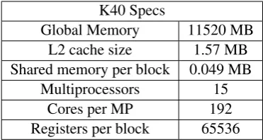
K40 Specs
Global Memory 11520 MB L2 cache size 1.57 MB Shared memory per block 0.049 MB
[image:2.595.323.509.62.161.2]Multiprocessors 15 Cores per MP 192 Registers per block 65536 Table 1: Device properties of a K40c GPU
The memory hierarchy on the device is laid out to maximize the data throughput. Table 1 shows the amount of cores available for execution as well as the amount of memory available on a Kepler based GPU. Registers are the fastest type of mem-ory on the device, and this memmem-ory is private to each thread running on a block. Shared memory is the second fastest, and is shared by all threads run-ning in the same block. The next type of memory is the L2 cache, which is shared among all stream-ing multiprocessors. The slowest and largest type of memory is global memory. Directly reading and writing to global memory affects performance sig-nificantly. Efficient memory management (reading and writing to and from contiguous addresses in memory) is important to fully utilize the memory hierarchy and increase performance.
2.2 Optimizations
Different factors such as number of threads in a block or coalesced memory accesses affect the performance on the GPU. In this section, we will cover the methods and modifications we used to improve the performance of our parallel imple-mentations.
multiprocessor must execute 12 warps total where 1 warp gets executes at a time in parallel.
In our implementations, we take the following approach. The number of cores per multiproces-sor is considered first to configure the block size. The block size is set to contain the same number of threads as the number of cores per multiproces-sor of the graphics card used. If the number of threads needed to perform a computation is not di-visible by the amount of cores per multiprocessor, the number of threads is rounded up to the clos-est dividend. Once the block size and number of threads are selected, the number of blocks is cho-sen by dividing the total number of threads by the block size.
Coalesced memory accesses are essential to maximize the use of resources running on the GPU. When data is requested by a warp execut-ing on a streamexecut-ing multiprocessor, a block from global memory will be accessed and allocated in shared memory. It is crucial to coalesce mem-ory accesses so the number of blocks of global memory requested and the global memory access times decrease. This can be achieved by making all threads in a warp access contiguous spaces in memory. A similar speedup can be achieved if each thread in a block allocates all the data re-quired from global memory into a compact data structure allocated in shared memory (size of the shared memory varies across devices). Section 4 describes the data structure used to coalesce mem-ory reads. For each input symbol wt the source states of all possible transitions can be read in a coalesced form and stored in shared memory al-lowing faster execution times.
Using special function units on the device can inhibit the performance of a program running on the GPU. Performance is affected because the number of SFU is lower than the amount of regular cores (e.g. The GK104 Kepler architecture con-tains 1536 regular cores and 256 special function units total). Also, the cycle penalty for using SFU rather than CUDA cores is higher than the penalty for regular cores on the device. For this work, the amount of instructions that use a specific SFU are kept to a minimum to obtain a higher speedup. By combining the mentioned techniques in this sec-tion, an application can significantly increase its performance.
3 Weighted Finite Automata
In this section, we review weighted finite au-tomata, using a matrix formulation. Aweighted fi-nite automatonis a tupleM=(Q,Σ,s,F, δ), where
• Qis a finite set of states.
• Σis a finite input alphabet.
• s ∈RQ is a one-hot vector: ifMcan start in stateq, thens[q]=1; otherwise,s[q]=0.
• f ∈RQis a vector of final weights: ifMcan accept in stateq, then f[q] > 0 is the weight incurred; otherwise, f[q]=0.
• δ : Σ → RQ×Q is the transition function: if
M is in state qand the next input symbol is
a, then δ[a][q,q0] is the weight of going to
stateq0.
Note that we currently do not allow transitions on empty strings or epsilon transitions. This defi-nition can easily be extended to weighted finite transducers by augmenting the transitions with output symbols. See Figure 1 for an example FST. Using this notation, the total weight of a string
w=w1· · ·wncan be written succinctly as:
weight(w)= s>
n
Y
t=1
δ[wt]
f. (1)
Matrix multiplication is defined in terms of multi-plication and addition of weights. It is common to redefine weights and their multiplication/addition to make the computation of (1) yield various use-ful values. When this is done, multiplication is often written as⊗and addition as⊕. If we define
p1⊗p2= p1p2andp1⊕p2 = p1+p2, then equation
(1) gives the total weight of the string.
Or, we can make Equation (1) obtain the maxi-mumweight path as follows. The weight of a tran-sition is (p,k), where p is the probability of the transition andkis (a representation of) the transi-tion itself. Then
(p1,k1)⊗(p2,k2)≡(p1p2,k1k2)
(p1,k1)⊕(p2,k2)≡((pp1,k1) ifp1 > p2 2,k2) otherwise.
0
1
2
3
4
5
le:the/0.48 le:a/0.08
chat:cat/1
chat:cat/1
</s>
:</s>/1
</s>:</s>
/1
Figure 1: Example of a FST that translates the french stringle chatto English.
4 Serial Algorithm
Applications of finite automata use a variety of al-gorithms, but the most common are the Viterbi, forward, and backward algorithms. Several of these automata algorithms are related to one an-other and used for learning and inference. Speed-ing up these algorithms will allow faster trainSpeed-ing and development of large scale machine learning systems.
The forward and backward algorithms are used to compute weights (Eq. 1), in left-to-right (Read-ing an input utterance from left to right) and right-to-left order, respectively. Their intermediate val-ues are used to compute expected counts dur-ing traindur-ing by expectation-maximization (Eisner, 2002). They can be computed by Algorithm 2.
Algorithm 1 is one way of computing Viterbi using Equation (1). It is a straightforward algo-rithm, but the data structures require a brief expla-nation.
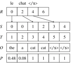
[image:4.595.90.281.61.126.2]Throughout this paper, we use zero-based in-dexing for arrays. Letm=|Σ|, and number the in-put symbols inΣconsecutively 0, . . . ,m−1. Then we can think ofδas a three-dimensional array. In general, this array is very sparse. We store it using a combination of compressed sparse row (CSR) format and coordinate (COO) format, as shown in Figure 2 where:
• z is the number of transitions with nonzero weight
• Ris an array of length (m+1) containing off -sets into the arraysS,T,O, and P. ifa ∈ Σ, the transitions on inputacan be found at po-sitionsR[a], . . .R[a+1]−1 (i.e. to access all transitionsδ[a] ). Note thatR[m]=z
• S contains the source states for each transi-tion 0≤k<z∈δ[a]
• T contains target states for transitions 0 ≤
k<z∈δ[a]
le chat </s>
R 0 2 4 6
S 0 0 1 2 3 4
T 1 2 3 4 5 5
O the a cat cat </s> </s>
[image:4.595.348.495.69.199.2]P 0.48 0.08 1 1 1 1
Figure 2: CSR/COO representation of FST in Fig-ure 1.
• Ocontains the output symbols for transitions from stateS[k] to stateT[k]
• P contains the probabilities for transitions from stateS[k] to stateT[k]
The vector f of final weights is stored as a sparse vector: for eachk,Sf[k] is a final state with weightPf[k].
Algorithm 1 Serial Viterbi algorithm (using CSR/COO representation).
1: forq∈Qdo 2: α[0][q]=0 3: α[0][s]=1 4: fort=1, . . . ,ndo 5: a←wt
6: fork=R[a], . . . ,R[a+1]−1do 7: p←α[t−1][S[k]]⊗P[k] 8: α[t][T[k]]←α[t][T[k]]⊕p 9: returnLkα[n][Sf[k]]⊗Pf[k]
If the transition matricesδ[a] are stored in com-pressed sparse row (CSR) format, which enables efficient traversal of a matrix in row-major order, then these algorithms can be written out as Algo-rithm 2 for the forward-backward algoAlgo-rithm and 1 for Viterbi. (Using compressed sparse columns (CSC) format, the loop over q0 would be outside
the loop over q, which is perhaps the more com-mon way to implement these algorithms.)
5 Parallel Algorithm
Algorithm 2Forward-Backward algorithm (row-major).
1: forward[0][s]←1 .Begin forward pass
2: fort=0, . . . ,n−1do 3: forq∈Qdo
4: forq0∈Qsuch thatδ[wt+1][q,q0]>0do
5: p=forward[t][q]δ[wt+1][q,q0]
6: forward[t+1][q0]+= p
7: forq∈Qdo .backward pass 8: backward[n][q]= f[q]
9: fort=n−1, . . . ,0do 10: forq∈Qdo
11: forq0∈Qsuch thatδ[wt+1][q,q0]>0do 12: p=δ[wt+1][q,q0]backward[t][q0]
13: backward[t][q]+= p 14: Z=Pq∈Qforward[n][q]f[q]
15: fort=0, . . . ,n−1do 16: forq,q0∈Qdo
17: α=forward[t][q] .Expected counts
18: β=backward[t+1][q0]
19: count[q,q0]+=α×δ[w][q,q0]×β/Z
are stored in CSR/COO format as described above for Algorithm 1. TheS,T, andParrays are stored on the GPU in global memory; theRandOarrays are kept on the host. For each input symbola, the transitions on S andT are sorted first by source state and then by target state; this improves mem-ory locality slightly. For the forward-backward algorithm, sorting by target improves the perfor-mance for the backward pass since the input is read from right to left.
For each input symbol wt, one thread is launched per transition, that is, for each nonzero entry of the transition matrixδ[wt]. Equivalently, one thread is launched for each transitionk such that R[wt] ≤ k < R[wt + 1], for a total of
R[wt +1]−R[wt] threads. Each thread looks up
q =S[k],q0 = T[k] and computes its
correspond-ing operation.
For example, in Figure 2, input word “le” has index 0; sinceR[0]=0 andR[1]= 2, two threads are launched, one fork=0 (that is, 0−−−−−−−−→le:the/0.48 1) and one fork=1 (that is, 0−−−−−−→le:a/0.08 2).
5.1 Viterbi
At the time of computing a transitionδ[wt][q,q0], if the probability (at line 8 in Algorithm 1) is higher than α[t][q0], we store the probability in
α[t][q0]. Because this update potentially involves
concurrent reads and writes at the same memory location, we use an atomic max operation (defined
asatomicMaxon the NVIDIA toolkit). However,
atomicMax is not defined for floating-point
val-ues. Additionally, this update needs to store a back-pointer (k) that will be used afterwards to re-construct the highest-probability path. The prob-lem is that theatomicMax provided by NVIDIA can only update a single value atomically.
We solve both problems with a trick: pack the Viterbi probability and the back-pointer into a single 64-bit integer, with the probability in the higher 32 bits and the back-pointer in the lower 32 bits. In IEEE 754 format, the mapping between nonnegative real numbers and their bit representa-tions (viewed as integers) is order-preserving, so a max operation on this packed representation up-dates both the probability and the back-pointer si-multaneously.
The reconstruction of the Viterbi path is not par-allelizable, but is done on the GPU to avoid copy-ingαback to the host avoiding a slowdown. This generates a sequence of transition indices, which is moved back to the host. There, the output sym-bols can be looked up in arrayO.
5.2 Forward-Backward
The forward and backward algorithms 2 are sim-ilar to the Viterbi algorithm, but do not need to keep back-pointers. In the forward algorithm, when a transitionδ[wt][q,q0] is processed, we up-date the sum of probabilities reaching state q0 in
forward[t+1][q0]. Likewise, in the backward
al-gorithm, we update the sum of probabilities start-ing fromqinbackward[t][q]. Both passes require atomic addition operations, but because we use log-probabilities to avoid underflow, the atomic addition must be implemented as:
log(expa+expb)=b+log1p(exp(a−b)), (2)
assuminga≤band where log1p(x)=log(1+x), a common function in math libraries which is more numerically stable for smallx.
We implemented an atomic version of this log-add-exp operation. The two transcenden-tals are expensive, but CUDA’s fast math option
(-use_fast_math) speeds them up somewhat by
6 Other Approaches
6.1 Parallel prefix sum
We have already mentioned a line of work begun by (Ladner and Fischer, 1980) for unweighted, nondeterministic finite automata, and continued by (Hillis and Steele, 1986) and (Mytkowicz et al., 2014) for unweighted, deterministic finite au-tomata. These approaches useparallel prefix sum
to compute the weight (1), multiplying each adja-cent pair of matrices in parallel and repeating until all the matrices have been multiplied together.
This approach could be combined with ours; we leave this for future work. A possible issue is that matrix-vector products are replaced with slower matrix-matrix products. Another is that prefix sum might not be applicable in a more general setting – for example, if a FST is composed with an input lattice rather than an input string.
6.2 Matrix libraries
The formulation of the Viterbi and forward-backward algorithms as a sequence of matrix mul-tiplications suggests two possible easy implemen-tation strategies. First, if transition matrices are stored as dense matrices, then the forward algo-rithm becomes identical to forward propagation through a rudimentary recurrent neural network. Thus, a neural network toolkit could be used to carry out this computation on a GPU. However, in practice, because our transition matrices are sparse, this approach will probably be inefficient.
Second, off-the-shelf libraries exist for sparse matrix/vector operations, like cuSPARSE.1
How-ever, such libraries do not allow redefinition of the addition and multiplication operations, making it difficult to implement the Viterbi algorithm or use log-probabilities. Also, parallelization of sparse matrix/vector operations depends heavily on the sparsity pattern (Bell and Garland, 2008), so that an off-the-shelf library may not provide the best solution for finite-state models of language. We test this approach below and find it to be several times slower than a non-GPU implementation. 7 Experiment
7.1 Setup
To test our algorithm, we constructed a FST for rudimentary French-to-English translation. We trained different unsmoothed bigram language
1http://docs.nvidia.com/cuda/cusparse/
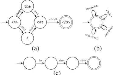
<s> the
a
cat </s>
the/
0.8
a/0.2 cat
/1
cat/
1
</s>/1
the:le/0.6 a:le
/0.4
cat: chat
/1
</s>:</s>
/1
(a) (b)
le chat </s>
[image:6.595.322.509.63.187.2](c)
Figure 3: Example automata/transducers for (a) language model (b) translation model (c) input sentence. These three composed together form the transducer in Figure 1.
models on 1k/10k/100k/150k lines of French-English parallel data from the Europarl corpus and converted it into a finite automaton (see Figure 3a for a toy example).
GIZA++was used to word-align the same data and generate word-translation tables P(f | e) from the word alignments, as in lexical weight-ing (Koehn et al., 2003). We converted this table into a single-state FST (Figure 3b). The language model automaton and the translation table trans-ducer were intersected to create a transtrans-ducer simi-lar to the one in Figure 1.
For more details about the transducers (number of nodes, edges, and percentage of non-zero ele-ments on the transducer) see Table 4.
We tested on a subset of 100 sentences from the French corpus with lengths of up to 80 words. For each experimental setting, we ran on this set 1000 times and report the total time. Our exper-iments were run on three different systems: (1) a system with an Intel Core i7-4790 8-core CPU and an NVIDIA Tesla K40c GPU, (2) a system with an Intel Xeon E5 16-core CPU and an NVIDIA Titan X GPU, and (3) a system with an Intel Xeon E5 24-core CPU and an NVIDIA Tesla P100 GPU.
7.2 Baselines
We compared against the following baselines:
Carmelis an FST toolkit developed at USC/ISI.2
OpenFST is a FST toolkit developed by Google as an open-source successor of the AT&T Finite State Machine library (Allauzen et al., 2007). For compatibility, our implementations read the Open-FST/AT&T text file format.
0 0.02 0.04 0.06 0.08 0.1 0.12
0 10 20 30 40 50 60 70 80
tim
e
(
s
)
Number of input words
Parallel Viterbi CuSPARSE Serial Viterbi
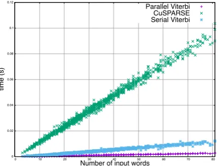
Figure 4: Viterbi decoding times for 1000 individ-ual test sentences compared for our serial, parallel, and cuSPARSE implementations (Titan X).
Our serial implementation Algorithm 1 for Viterbi and Algorithm 2 for forward-backward.
cuSPARSE was used to implement the forward algorithm, using CSR format instead of COO for transition matrices. Since we can’t redefine addi-tion and multiplicaaddi-tion, we could not implement the Viterbi algorithm. To avoid underflow, we rescaled the vector of forward values at each time step and kept track of the log of the scale in a sep-arate variable.
To be fair, it should be noted that Carmel and OpenFST are much more general than the other implementations listed here. Both perform FST composition in order to decode an input string adding another layer of complexity to the process. The timings for OpenFST and Carmel on Table 2 include composition
7.3 Results
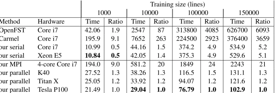
Table 2 shows the overall performance of our Viterbi algorithm and the baseline algorithms. Our parallel implementation does worse than our se-rial implementation when the transducer used is small (presumably due to the overhead of kernel launches and memory copies), but the speedups increase as the size of the transducer grows, reach-ing a speedup of 5x. The forward-backward algo-rithm with expected counts obtains a 5x speedup over the serial code on the largest transducer (See Table 3).
CuSPARSE does significantly worse than even our serial implementation; presumably, it would have done better if the transition matrices of our
[image:7.595.73.288.64.227.2]transducers were sparser.
Figure 4 shows decoding times for three algo-rithms (our serial and parallel Viterbi, and cuS-PARSE forward) on individual sentences. It can be seen that all three algorithms are roughly linear in the sentence length.
Viterbi is faster than either the forward or back-ward algorithm across the board. This is because the latter need to add log-probabilities (lines 6 and 13 of Algorithm 2), which involves expensive calls to transcendental functions.
7.4 Comparison across GPU architectures
Table 2 compares the performance of the Kepler-based K40, where we did most of our experiments, with the Maxwell-based Titan X and the Pascal-based Tesla P100. The performance improvement is due to different factors, such as a larger num-ber of active thread blocks per streaming multipro-cessor on a GPU architecture, the grid and block size selected to run the kernels, and memory man-agement on the GPU. After the release of the Ke-pler architecture, the Maxwell architecture intro-duced an improved workload balancing, reintro-duced arithmetic latency, and faster atomic operations. The Pascal architecture allows speedups over all the other architectures by introducing an increased floating point performance, faster data movement performance (NVLink), larger and more efficient shared memory, and improved atomic operations. Also, SMs on the pascal architecture are more efficient allowing speedups larger speedups than its predecessors. Our parallel implementations were compiled using architecture specific flags
(-arch=compute_XX) to take full advantage of
the architectural enhancements described in this section.
7.5 Comparison against a multi-core implementation
Training size (lines)
1000 10000 100000 150000
[image:8.595.81.523.62.211.2]Method Hardware Time Ratio Time Ratio Time Ratio Time Ratio OpenFST Core i7 42.06 1.9 2547 87 313800 4085 626700 6093 Carmel Core i7 195.9 9.1 7652 263 224500 2923 376400 3659 our serial Core i7 10.99 0.5 44.16 1.5 374.2 4.9 534.9 5.2 our serial Xeon E5 10.84 0.5 42.05 1.4 375.3 4.9 529.6 5.1 our MPI 4-core Core i7 194.0 9.0 581.2 20 1849 24 2243 21 our parallel K40 27.52 1.3 38.26 1.3 116.5 1.5 131.1 1.3 our parallel Titan X 25.05 1.2 33.92 1.2 94.07 1.2 121.6 1.2 our parallel Tesla P100 21.49 1.0 29.04 1.0 76.79 1.0 102.9 1.0
Table 2: Our GPU implementation of the Viterbi algorithm outperforms all others tested on the medium and large FSTs. Times (in seconds) are for decoding a set of 100 examples 1000 times using Viterbi. Ratios are relative to our parallel algorithm on the Tesla P100.
Training size (lines)
method 1k 10k 100k 150k
cuSPARSE forward 646 1846 3555 5948 serial forward 36 251 2297 3346 parallel forward 17 37 236 327
serial backward 13 248 3585 5303 parallel backward 43 80 644 1070
serial combined 47 534 6065 8790 parallel combined 60 120 1111 1773
Table 3: Our GPU implementations of the forward and backward algorithms, and for-ward+backward+expected counts combined, out-perform all others tested, on the medium and large FSTs. Times (in seconds) are for processing 100 examples 1000 times, on a Core i7 and K40.
Training size States Transitions Non-zero
1000 3505 443527 3.6%
10000 11644 6792487 5.0% 100000 33125 95381368 8.7% 150000 39420 150971615 9.7%
Table 4: FST Comparison. This table shows the number of states, edges, and percent of non zero elements of the transducers created using 1k/10k/100k/150k examples.
since all the memory is already on the graphics card and the cost of using global memory on the GPU is lower than synchronizing and sharing data between cores.
8 Conclusion
We have shown that our algorithm outperforms several serial implementations (our own serial im-plementation on a Intel Core i7 and Xeon E ma-chines, Carmel and OpenFST) as well as a GPU implementation using cuSPARSE.
A system with newer and faster cores might achieve higher speedups than a GPU on smaller datasets. However,building a multi-core system that beats a GPU setup can be more expensive. For example, a 16 core Intel Xeon E5-2698 V3 can cost 3,500 USD (Bogoychev and Lopez, 2016). Newer GPU models offer previous generation CPU’s the opportunity to obtain speedups for a lower price (Titan X GPUs sell cheaper than Xeon E5 setups at US$1,200). Speeding up computation on a GPU would allow users to speed up applica-tions cheaper without investing on a newer multi-core system.
Our implementation has been open-sourced and is available online. 3 In the future, we plan to
ex-pand this software into a toolkit that includes other algorithms needed to run a full machine translation system.
Acknowledgements
This research was supported in part by a gift of a Tesla K40c GPU card from NVIDIA Corporation.
3https://bitbucket.org/aargueta2/
[image:8.595.73.291.310.435.2]References
Cyril Allauzen, Michael Riley, Johan Schalkwyk, Wo-jciech Skut, and Mehryar Mohri. 2007. OpenFst: A general and efficient weighted finite-state trans-ducer library. InProc. International Conference on Implementation and Application of Automata (CIAA
2007), pages 11–23.
Nathan Bell and Michael Garland. 2008. Effi -cient sparse matrix-vector multiplication on CUDA. Technical Report NVIDIA Technical Report NVR-2008-004, NVIDIA Corporation.
Nikolay Bogoychev and Adam Lopez. 2016. N-gram language models for massively parallel devices. In
Proc. ACL, pages 1944–1953.
John Canny, David Hall, and Dan Klein. 2013. A multi-teraflop constituency parser using GPUs. In
Proc. EMNLP, pages 1898–1907.
Jike Chong, Ekaterina Gonina, Youngmin Yi, and Kurt Keutzer. 2009. A fully data parallel WFST-based large vocabulary continuous speech recognition on a graphics processing unit. InProc. INTERSPEECH, pages 1183–1186.
Jason Eisner. 2002. Parameter estimation for proba-bilistic finite-state transducers. InProc. ACL, pages 1–8.
David Hall, Taylor Berg-Kirkpatrick, and Dan Klein. 2014. Sparser, better, faster GPU parsing. InProc. ACL, pages 208–217.
Hua He, Jimmy Lin, and Adam Lopez. 2013. Mas-sively parallel suffix array queries and on-demand phrase extraction for statistical machine translation using gpus. InProc. NAACL HLT, pages 325–334. W. Daniel Hillis and Guy L. Steele, Jr. 1986. Data
parallel algorithms. Communications of the ACM, 29(12):1170–1183.
Jungsuk Kim, Jike Chong, and Ian R Lane. 2012. Ef-ficient on-the-fly hypothesis rescoring in a hybrid gpu/cpu-based large vocabulary continuous speech recognition engine. InProc. INTERSPEECH, pages 1035–1038.
Philipp Koehn, Franz Josef Och, and Daniel Marcu. 2003. Statistical phrase-based translation. InProc.
NAACL HLT, pages 48–54.
Shankar Kumar, Yonggang Deng, and William Byrne. 2005. A weighted finite state transducer translation template model for statistical machine translation.
J. Natural Language Engineering, 12(1):35–75.
Richard E. Ladner and Michael J. Fischer. 1980. Par-allel prefix computation.J. ACM, 27(4):831–838. John D. Lafferty, Andrew McCallum, and Fernando
C. N. Pereira. 2001. Conditional random fields: Probabilistic models for segmenting and labeling se-quence data. InProc. ICML, pages 282–289.
Rongchun Li, Yong Dou, and Dan Zou. 2014. Efficient parallel implementation of three-point viterbi decod-ing algorithm on CPU, GPU, and FPGA.
Concur-rency and Computation: Practice and Experience,
26(3):821–840.
Duane Merrill, Michael Garland, and Andrew Grimshaw. 2012. Scalable GPU graph traver-sal. In Proc. 17th ACM SIGPLAN Symposium on Principles and Practice of Parallel Programming
(PPoPP), pages 117–128.
Mehryar Mohri, Fernando C. N. Pereira, and Michael Riley. 2002. Weighted finite-state transducers in speech recognition. Computer Speech and
Lan-guage, 16(1):69–88.
Mehryar Mohri. 2009. Weighted automata algo-rithms. In Manfred Droste, Werner Kuich, and Heiko Vogler, editors, Handbook of Weighted
Au-tomata, pages 213–254. Springer.
Todd Mytkowicz, Madanlal Musuvathi, and Wolfram Schulte. 2014. Data-parallel finite-state ma-chines. InProc. Architectural Support for
Program-ming Languages and Operating Systems (ASPLOS),
March.
Veynu Narasiman, Michael Shebanow, Chang Joo Lee, Rustam Miftakhutdinov, Onur Mutlu, and Yale N Patt. 2011. Improving GPU performance via large warps and two-level warp scheduling. In Proc.
IEEE/ACM International Symposium on
Microarchi-tecture, pages 308–317.
Hao Peng, Rongke Liu, Yi Hou, and Ling Zhao. 2016. A Gb/s parallel block-based viterbi decoder for convolutional codes on gpu. arXiv preprint
arXiv:1608.00066.