Abstract- This paper presents the recognition of shapes for object
retrieval in image databases using skeleton-based and contour-based representation by discrete curve evaluation and two consecutive primitive edges. Humans tend to use high-level concepts in everyday life. Object segmentation and recognition is the primary step of computer vision to achieve image retrieval of high-level image analysis. Contour-based and skeleton-based representations are important for object recognition in different areas. In comparing the contour-based approaches with the skeleton-based approaches for object representation, the contour-based is more sensitive to noise than a skeleton-based approach based on a good skeleton pruning method, but a rough shape classification can be performed since the obtained skeletons do not represent any shape details. In this paper, we proposed a novel method to integrate the contour-based approaches with skeleton-based approaches for object representation. The contour-based and skeleton-based representations are based on the proposal of two consecutive primitive edges method and discrete curve evolution method respectively. Experimental results demonstrate that the performance of the proposed algorithm is superior to Torsello and Hancock’s method [7] in terms of retrieval accuracy.
Index Terms:Keywords: Skeleton, shape similarity measure, visual parts, discrete curve evolution
I.
INTRODUCTIONIn the past, contour and skeleton were usually used to analyze and represent the shape of objects. Contour-based is an important aspect of human visual perception. Polygonal approximation has been a very popular shape representation technique. It not only satisfactorily represents a shape, but also significantly reduces the amount of processing data for further applications. Therefore, many shape recognition (matching) methods through polygonal approximation [1] have been proposed. However, some conventional methods are somewhat sensitive to non-consistent results of polygonal approximation. For example, the method [1] using attributed string matching cannot accurately define the edit distance (cost) for insertion and deletion operations. Latrcki and Lakamper [2] proposed a convexity rule for shape decomposition based on discrete contour evolution. They concentrate some of decomposition of 2D objects into meaningful visual parts and proposed a contour evaluation
Manuscript received January 3, 2009.
Tian-Luu Wu is with the Electronic Engineering, National Kinmen Institute of Technology, Taiwan, R.O.C. (corresponding author to provide phone: +886-82-313559; fax: +886-82-313304; e-mail:[email protected]).
Ji-Hwei Horng is with the Electronic Engineering, National Kinmen Institute of Technology, Taiwan, R.O.C. (e-mail:[email protected]).
method for identifying the visual part whether it is a significant convex part or not.
The skeleton is another important method for object representation and recognition. Skeleton-based representations are the abstractions of objects, which contain both shape features and topological structures of original objects. Many researchers have made efforts to recognize the generic shape by matching skeleton structures represented by graphs or trees [3]. Unfortunately, these approaches have only demonstrated the applicability to objects with simple and distinctive shapes, and therefore, cannot be applied to more complex shapes like shapes in a MPEG-7 data set.
The most common approaches for overcoming skeleton instability are based on skeleton pruning. Pruning can either be performed implicitly as a post processing step or integrated in the step of skeletonization computation. In general, the skeletonization algorithms can broadly be classified into four types: (1) the first type is thinning algorithms, such as those with shape thinning and the wave front/grassfire transform. These algorithms iteratively remove border points, or move to the inner parts of an object in determining an object’s skeleton; (2) the second type is the category of discrete domain algorithms based on the Voronoi diagram. These methods search the locus of centers of the maximal disks contained in the polygons with vertices sampled from the boundary; (3) the third type of algorithms is to detect ridges in a distance map of boundary points. Approaches based on distance maps usually ensure accurate localization but does not guarantee that the skeleton can connect completely; (4) the fourth type of algorithms is based on mathematical morphology. Usually, these methods can localize the accurate skeleton, but may not guarantee the connectivity of the skeleton.
In this paper, we proposed a method to integrate the contour-based approaches with skeleton-based approaches for object representation. The contour-based and skeleton-based approaches are based on the proposed two consecutive primitive edges method and the discrete curve evolution method respectively. To overcome skeleton instability based on skeleton pruning, the proposed skeleton pruning approaches can prune the redundant skeleton branches based on the contour estimation and pre-selection of the implicit skeleton branches.
II.
SKELETON GROWING WITH CONTOURINFORMATION
A. The Proposed Contour Sampling Method using Discrete
Recognition of Shapes for Object Retrieval in
Image Databases by Discrete Curve Evolution and
Two Consecutive Primitive Edges
Curve Evolution
GHT [4] was initially proposed to represent a planar set D with arbitrary boundary using a so-called R-table [4]. As an example shown in Fig. 1, the boundary of the planar set D can be described by geometric relationship between the centroid XR of D and the boundary point X’s. According to the R-table in GHT to represent the boundary in question can be constructed as:
). , ( ),..., , ( ), , (
), , ( ),..., , ( ), , (
), , ( ),..., , ( ), , (
), , ( ),..., , ( ), , (
3 3 2 2 1 1
3 3 3 3 2 3 2 3 1 3 1 3 3
1 2 1 2 2 2 2 2 1 2 1 2 2
1 1 1 1 2 1 2 1 1 1 1 1 1
n k n k k k k k k
n n
n n
n n
r r
r
r r
r
r r
r
r r
r
α α
α φ
α α
α φ
α α
α φ
α α
α φ
#
(1)
where φi is the common slope for the tangent line passing
through the boundary points xij,j=1,...,n. However, the
information of R-table in GHT cannot link information of boundary into the planar set D in an image, and it is also difficult to express which boundary is a significant visual part.
The characters of significant visual part in a contour have be proposed in literature [5]. We can summarize the observation into four rules:
(1) These visual parts are defined to be “convex” or “nearly convex shape” from the rest of object at concavity extrema.
(2) Although the observation that visual parts are “nearly convex shapes” is very natural. The main problem is to determine the meaning of “nearly” in this context. (3) Many significant visual parts are not convex in the
mathematic sense, since a visual part may have small concavities, e.g., small concavities caused by fingers of the human hand.
(4) The role of each visual part in any object is different from the sense of human vision, e.g., the perpendicular angle is less than the straight line in a square shape. If the perpendicular angle is loss then it cannot form a square. On the opposite view, increasing or decreasing the straight lines, will still maintain the square. In this respect, the smaller number of visual parts is more significant than the larger number of visual parts. To estimate the “significant” visual part in a whole object is a difficult task without a prior knowledge about the boundary of objects or without user interactive. Our solution is using a hierarchical evolution rule which includes two stages: (1) estimate the turning point of visual parts based on the chain-code method and discrete curve evolution; (2) select the visual part into significant visual parts from all of visual parts in an object.
First, we propose a contour sampling method for estimating the turning point of visual parts based on chain-code method. In the chain-code process, the point coded moves along the digital curve or edge pixels with 8-adjacency model in 8-direct code. This assumes that the chain-code with 8-adjacency in a 3×3 block is limited to a multiple of 450 and it is quantized to be the nearest multiple
of 450. A boundary chain starts with a random point in the edge pixels. Each edge pixel has 8 neighboring points among which there is at least one edge point. The boundary chain-code is the direction description of current point aj to the next one aj+1, and the chain-code can be defined as
ej =aj →aj+1 (2) where ej denotes the number 0 to 7 for a description in 8-direction chain-code.
XR
X r
φ α
[image:2.595.335.515.182.270.2]x y
Fig. 1.The coordinated relationship between a boundary point X and the centroid XR of an object with arbitrary shape.
ei ei+1
(g)
aj aj+1 aj+2 aj aj+1 aj+2 ei ei+1
aj aj+1 aj+2 ei
ei+1
(a) (b) (c)
aj+2
aj ei aj+1 ei+1
aj+2 aj aj+1
ei ej+1 ei
aj aj+1
aj+2 e j+1
(d) (e) (f)
aj aj+1
aj+2 ei ej+
1
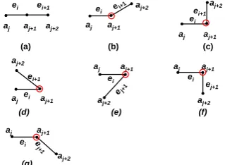
Fig.2 shows the possible 7 types of visual parts in a 3×3 block.
The boundary in a planar set D can be described with a start point and a series of sequence direction codes. There are some problems of chain-code method: (1) the chain-code varies dramatically with different start points. Selecting the proper start point on the chain-code is a common process; (2) the chain-code method cannot be applied to the rotation and scaling of D. Based on this reason, the consecutive primitive edge is proposed to describe the boundary of D. The concept of consecutive primitive edge φi is as follows:
φ
i=
|
e
i−
e
i−1|,
i
=
1
,...,
n
(3) where ei and ei-1 denote the consecutive primitive edges respectively. The detected of φi can be mapped to 7 types of visual parts, as shown in Fig.2. According to the key property of discrete curve evolution, a relevance measure k is given by
) 1 ( ) (
) 1 ( ) ( ) 1 , ( 1
)
,
(
+ +
+ +
+
=
j e j e
j e j e j e j e j
j
e
e
k
β A AA A (4) [image:2.595.345.505.311.428.2]of the curve of arc ej∪ej+1. Based on satisfying the rule (1-3) mentioned above, the turning point of visual part may appear as a (red) circle in Fig. 2 using the relevance measure k.
[image:3.595.311.556.76.458.2]The next problem is to find the significant visual part which hides in the boundary of an object. Mapping the consecutive primitive edge to a visual part is to encode an object with visual parts block by block along the boundary pixels. Hence, two given object blocks from along the edge pixel can be encoded and indicate which visual part is mapped, and the front of visual part ej+1 and the rear of visual part ej in Eq. (3) are overlapping. Without loss of generality, the histogram of consecutive primitive edge is used to describe the boundary of objects in this paper. Let CPEi,i=1,...,7denote the type of consecutive primitive edges and Ni is the number of CPEiin Fig. 2. The boundary of object BO will be described by
∑
≤ ≤ =
7 1 k k
N
BO (5)
For the CPE, the local significance of a boundary point is usually only considered and the global information of shape in an object is discarded. Assume that the arrangement of Nk in descending order (N1≤N2≤N3≤...≤N7) associates the same ordering to the CPEis
CPE1≤CPE2≤,...,≤CPE7 (6)
A ratio is decided to reserve how much of the visual parts can represent the object as the significant visual parts and the remainder will be ignored. The ratioρis defined by
∑ ≤ ≤
∑ ≤ ≤ ≤
7 1
1
j j
N p i i
N
ρ (7)
where p (p<7) denotes preceding sequences in eq. (7). It is important to determine a good stop criterion of the ratio selected. However, the ratio ρ selected usually appears in a variety of application-dependent cases. According to the experimental results, it can preserve the perceptual appearance sufficiently for object recognition when the ratioρ is assigned as 0.1.
A skeleton similarity measure is useful for object-based retrieval in image databases should be according to our perception. This basic property leads to the following requirements:
(1) A skeleton similarity measure shall permit recognition of perceptually similar objects that are not mathematically identical.
(2) It shall preserve significant visual parts of objects.
(3) It shall not depend on scale, orientation, or position of objects.
(4) A skeleton similarity measure is universal, in the sense that it allows us to identify or distinguish objects of arbitrary skeleton, i.e. no restrictions on shapes are assumed.
We should further introduce the skeleton growing based on following rules.
Rule 1. Let the boundary ∂D of a set D be composed of k simple contour segments C1, C2, …,Ck. Let T1, T2,…,Tn be the turning points lying on the simple contour segment,
which were selected using Eq. (7). The turning point set Ti also generated a skeleton branch.
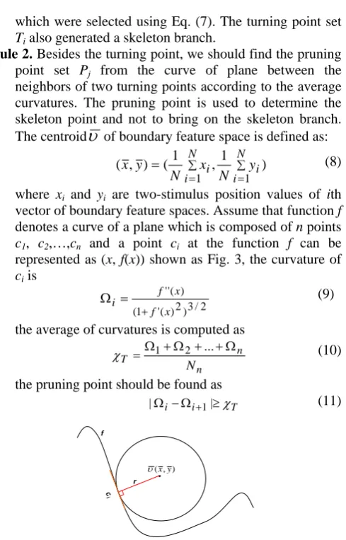
Rule 2. Besides the turning point, we should find the pruning point set Pj from the curve of plane between the neighbors of two turning points according to the average curvatures. The pruning point is used to determine the skeleton point and not to bring on the skeleton branch. The centroid
υ
of boundary feature space is defined as:( , ) (1 , 1 )
1 1
∑ = ∑ =
= N
i i N
i i
y N x N y
x (8)
where xi and yi are two-stimulus position values of ith vector of boundary feature spaces. Assume that function f denotes a curve of a plane which is composed of n points c1, c2,…,cn and a point ci at the function f can be represented as (x, f(x)) shown as Fig. 3, the curvature of ci is
2 / 3 ) 2 ) ( ' 1 (
) ( ''
x f
x f i
+ =
Ω (9)
the average of curvatures is computed as
n n T
N Ω + + Ω + Ω
= 1 2 ...
χ (10)
the pruning point should be found as
|Ωi−Ωi+1|≥χT (11)
r f
c
i
) ,
(xy
[image:3.595.316.554.267.458.2]υ
Fig. 3 shows the curvatureΩof a point ci at the function f.
Rule 3. If a straight boundary is between the neighbors of two turning points, then the pruning point is determined using the center of the straight boundary.
Rule 4. The skeleton should be grown according to the boundary points set ℜ of the object, which include turning points set Ti and pruning points set Pj, and defined as ℜ={{Ti}∪{Pj)},i=1,...,n,j=1,...,m.
Rule 5. Connect skeleton points which are found using the boundary point set ℜ and turning points Ti’s, the skeleton arc of the object is found.
B. Skeleton Growing
Assume that ai-1, ai, and ai+1 denote two consecutive points, and the ai is a turning point which belongs to the set of Ti. The boundary segments between ai-1and ai, and ai and ai+1 can be represented as ax+by+c=0 and dx+ey+f=0, respectively, where a, b, c, d, e, and f denote the parameters of boundary segments. It should find the auxiliary line L which connects point ai-1 and ai+1 shown as Fig.4. Let
θ
denote an included angle between the line ax+by+c=0 and dx+ey+f =0. That is2
1 θ
θ
2 2
2 2
2 1
tan tan 1
tan tan
) tan( tan
θ θ
θ θ
θ θ θ
− + =
− =
(13)
Let
2
tanθ
=
x , it will be computed as
) (
) ( 2 ) ( 2
tan
ae bd
ae bd be ad
x
=
θ=
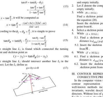
− + +− − (14)According to the
2 1 θφ θ
θ = + , it is simple to prove
2 tan 1 tan 1
2 tan 1 tan
2 1 ) tan(
tan θ
θ θ θ θ
φ
θ
θ
+ −
= −
= (15)
The straight line L1 is found which connected the turning point and skeleton point as
)
(
tan
)
(
y
−
y
1=
θ
φx
−
x
1 (16)The straight line L1 should intersect another line L2 in the object. Let the L2 define as
[image:4.595.55.412.83.420.2]gx+hy+i=0 (17)
Fig. 4. A skeleton point s is grown using the turning point ai.
Combining the equations (16) and (17), it is assumed that the homogeneous system has a nontrivial solution. The nontrivial solution of system should be found by performing of Guass-Jordan reduction procedure on the augmented matrix [M|0]. The result is
⎥ ⎦ ⎤ ⎢
⎣ ⎡
0 0
| |
1 0
0 1
2 1
k
k (18)
where ki,i=1,2 are the ratios of x and y. Based on the reduction results, the values of x2 and y2 has the intersect point between straight line L1 and L2, and can be computed as
) ,
( ) , (
2 2 2 1 1
2 2
2 2 1 1
1 2
2
k k
k k
k k
y x
+ + +
+
= (19)
The skeleton point should be found as
( , )
2 2 1 2
2
1 x y y
x
s= + + (20)
Based on the skeleton point sets
s
k,
k=n+m is found from the boundary points set ℜ of the object. The skeleton arc comes into being according to the following algorithm. Algorithm 1: Proposed the skeleton arc of object comes into being.Input: Two boundary point sets {Ti} and
m j n i P
Ti} { j)}, 1,..., , 1,...,
{{ ∪ = =
= ℜ
Output: A skeleton arc of the object comes into being. Method:
1. Let S denote the collection of all the skeleton point sets sk,
and empty initially.
2. Let E denote the completed skeleton arc of an object and empty initially.
3. while (ℜ≠NULL)
Find a skeleton point using a boundary point in ℜ by the equation (20).
Insert the skeleton point into S and delete the skeleton point fromℜ.
4. Select a skeleton point from S to E. 5. While (S≠NULL)
5.1. Find a skeleton point p from S, and its minimum distance isdmin(p.q), where q is a skeleton point in E.
5.2. Insert the skeleton arc into E and delete the skeleton from
ℜ
.6. While (T ≠NULL)
6.1. Find a skeleton point p from T, and its minimum distance is dmin(p.q), where q is a skeleton point in E. 6.2. Insert the skeleton branch into E and delete the
skeleton point from T.
III. CONTOUR REPRESENTATION BASED ON TWO CONSECUTIVE PRIMITIVE EDGES
In the computer vision there is a long history of work on contour representation and contour similarity. Some well-known methods include Fourier descriptor, moment invariants, wavelet descriptors and histogram of boundary directors. Without loss of generality, the histogram of CPE in Eq.(3) is used to describe the contour representation in this paper. For practical purposes, the histogram of CPE method cannot efficiently and correctly described the contour of an object. As shown in Fig. 2(c) and (f), the histogram of CPE is the same because it is a discrete primitive visual pattern. To solve this problem, the Eq.(3) is modified into two consecutive primitive edge Γ(α)as follows:
| |
|
| 1 1
1 )
(
j j j j j
j∪ =e −e ∪ e −e
=
Γα φ φ + − + or
| |
|
| 1 1
1 ) (
− +
+ ∪ = − ∪ −
=
Γα φj φj ej ej ej ej (21)
where∪denotes a union operation. Instead of representing a boundary in any possible combination, the detected two-consecutive primitive edge (TCPE) is mapped to 16 types of visual pattern as shown in Fig.5. The main reason for mapping the TCPE to virtual-pattern is to encode the boundary of an object with visual-pattern block by block along the edge pixels. Hence, two given object blocks from along the boundary pixel can be encoded and can indicate which visual-pattern is mapped. If we have a shape of an object such as Fig. 1, the R-table can be modified based on the proposed TCPE as
)) , , , ( , ( )),..., , , , ( , ( )), , , , ( ,
(Γ1α a0 a1a2 a3 Γ2α a2a3 a4 a5 Γnα an an+1a0 a1 (22)
where α is belonging to the type of virtual-pattern in Fig. 5, a0 and an denote the start-point and end-point respectively. To obtain the consistency of TCPE for any structure of objects, two decision rules are considered: (1) the starting boundary and ending boundary overlap; (2) the scanning sequence uses the anticlockwise method in the boundary of object.
REPRESENTATION
Consider a database DB consisting of a large number of objects. Each of them is represented as a high-dimensional feature vectorF ={Γ,Φ,β}, where Γ,Φ,andβ denote the feature vector of TCPE, skeleton arcs, and skeleton branch in an object, respectively. The feature vector of TCPE can further be represented asΓ={{fi,pj},i=1,...,16;j=1,...,n} , where fi and pjare ith feature and the corresponding number of TCPE in Fig. 6, respectively. The total number of TCPE in an object can be computed as
16 .
1 , ∑ = = i i j p ζ (23)
1 2 3 4
5 6 7 8
9 10 11 12
[image:5.595.361.550.131.257.2]13 14 15 16
Fig.5. Possible sixteen types of visual patterns in a square block. Let X={{xi,pk},k=1,...,16}and Y={{yj,qk},k=1,...,16}be the feature vectors of TCPE. Then the distance between X and Y based on the concept of QBIC [6] can be computed as j i i j i j j j i i TCPD x y p q a pq D ∑ = ∑= ∑ = ∑ = + − = 16 1 16 1 , 16 1 2 16 1 2 2 2 ) , ( (24)
where aij is the perceptual coefficient between feature values pk and qk. The role of each TCPE in any object is different from the sense of human vision. The fewer numbers of TCPE is more important than many numbers of TCPE in an object. Thus, the perceptual coefficient aijcan be defined as ∑ = ∑= + + = 16 1 16 1 1 1 1 1 , | | | | i j pi qj j q i p j i a (25)
where the values piand qj are assumed as non-zero, otherwise the corresponding value of 1/pi or 1/qj is assigned as zero. The feature vector of skeleton arcs can further be represented as β={{si,si+1,θi},i=1,...,n}shown as Fig. 6, where si and si+1 are the consecutive of skeleton arcs and θi denotes the included angle between the consecutive skeleton arcs siand si+1. A weight of skeleton arcs in an object can be found as ∑ = = n i sa i sa W W 1 (26)
and the sa i W is defined as 1 + + = i i i sa i s s W θ (27)
LetX={{sia,sia+1,θia},i=1,...,n}and Y={{sbj,sbj+1,θbj},j=1,...,m)be the feature vectors of skeleton arcs. Then the distance between X and Y is computed as Dsa =|WXsa−WYsa| (28)
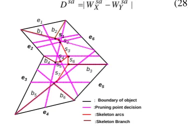
[image:5.595.81.292.214.351.2]: Boundary of object :Pruning point decision :Skeleton arcs :Skeleton Branch e1 e2 b1 b2 b3 b4 b5 b 6 s1 s2 s3 s4 s5 s6 s7 e3 e4 e5 e6 Fig. 6. An example of representing an object by the boundary of object, skeleton arcs, and skeleton branch. The feature vector of a skeleton branch can further be represented as φi={{ei,ej,bk},i,j=1,...,m,k=1,...,n}shown as Fig. 6, where bkdenotes the skeleton branch, and eiand ejare the boundary edges of object, which is connecting to the skeleton branch bk. A weight of a skeleton branch in an object can be found as ∑ = = n i sb i sb W W 1 (29)
and the sb i W is defined as ⎪ ⎩ ⎪ ⎨ ⎧ > > = i j j s i s j i i s j s sb k b s s when s s when W , , (30)
Let X ={{eix,exj,bkx},i,j=1,...,m1,k=1,...,n1} and } ,..., 1 , ,..., 1 , }, , , {{e e b l m m1 n n1 Y= ly my ny = = be the description vectors of a skeleton branch. Then the distance between X and Y is computed as Dsb=|WXsb−WYsb| (31)
between 0 and 1. The larger the value ofDs(X,Y), mean a greater similarity between the query object X to the database object Y. Combining the skeleton and contour features, the hybrid similarity measurement can be defined as
DTotal =β1⋅Ds(X,Y)+β2⋅D~TCPD (33) where DTotal is the value of hybrid similarity,
) , (X Y
Ds andD~TCPD are the values of similarity on the basis
of skeleton and contour features respectively, andβ1and β2
represent the weighting of Ds(X,Y)andD~TCPD, respectively. We should also setβ1+β2 =1.
V. EXPERIMENTAL RESULTS
In order to evaluate the proposed approach, a series of experiments were conducted on an Intel PENTIUM-IV 3GHz PC. A skeletal measure method proposed by Torsello and Hancock’s method [7] is also simulated by computer software for the purpose of performance comparison. An image database which consisted of 1266 binary objects is extracted from scenery images. Each object image in database is first formatted to 256×256 for testing the retrieval approach. Before the evaluation, human assessment was done to determine the relevant matches in the database to the query object image. The top 100 retrievals from both the Torsello and Hancock’s method and the proposed approaches were marked to decide whether they were indeed visually similar in skeleton and contour.
It is difficult to derive a formal method in evaluating the retrieval accuracy of an image database system. Traditional metrics for evaluating performance are recall and precision. They are functions of both correct matches and the relevance of database images to a query. The retrieval accuracy measured by recall and precision is computed as following. Recall measures the ability of the system to retrieval all the images that are relevant and defined as
relevances all
retrieved correctly
levances
call Re
Re = .
Precision measures the ability of the system to retrieve only images that are relevant and can be computed by
retrieved all
retrieved correctly
relevances
ecision=
Pr .
Recall and precision require a ground truth to assess the relevance of images for a set of significant queries.
The performance of the proposed image retrieval method is evaluated in terms of retrieval accuracy. The average precision and recall curves are plotted in Figs. 7(a) and 7(b), respectively. It can be seen that the proposed method achieves good results in terms of retrieval accuracy compared with Torsello and Hancock’s method [7].
VI. CONCLUSION
In this paper we have presented the recognition of shape-matching for object retrieval in image databases using skeleton and contour by discrete curve evaluation and two consecutive primitive edges. Object segmentation and recognition is the primary step of computer vision to achieve
image retrieval of high-level image analysis. Contour-based and skeleton-based representations are important for object recognition in different areas. In this paper, we proposed a novel method to integrate the contour-based approaches with skeleton-based approaches for object representation. The contour-based and skeleton-based representations are based on the proposed two-consecutive primitive edges method and discrete curve evolution method respectively. The experimental results demonstrate that the proposed method is superior to Torsello and Hancock’s method in terms of retrieval accuracy.
REFERENCES
[1]W. H. Tsai. And S. S. Yu, 1985, “Attributed string matching with merging for shape recognition,” IEEE Trans. PAMI, 7(4), pp. 453-462.
[2] L. J. Latecki and R. Lakamper, 1999, “Convexity Rule for shape Decomposition Based on Discrete Contour Evolution,” Computer Vision and Image Understanding, 73(3), pp. 441-454.
[3] C. D. Ruberto, 2004, “Recognition of shape by attributed skeletal graphs,” Pattern Recognition, 37, pp. 21-31. [4] S. C. Cheng, C. T. Kuo and H. J. Chen, 2007, “Visual
object retrieval via block-based visual-pattern matching,” Pattern Recognition, 40, pp. 1695-1710.
[5] L. J. Latecki and R. Lakamper, 1999, “ Convexity Rule for Shape Decomposition Based on Discrete Contour Evolution,” Computer Vision and Image Understanding, 73, pp.441-454.
[6] M. flickner, H. Sawhney, W. Niblack, J. Ashley, Q. Huang, B. Dom, M. Gorkani, J. Hafner, D. Lee, D. Petkovic, D. Steele, and P. Yanker,” Query by image and video content: the QBIC system, IEEE Computer, 28(9), pp23-32, 1995. [7] A. Torsello and E. R. Hancock, 2004,” A Skeletal measure
of 2D shape similarity,” Computer Vision and Image Understanding, 95, pp. 1-29.
10 20 30 40 50 60 70 80 90 100
0.1 0.2 0.3 0.4 0.5 0.6 0.7 0.8
Number of retrievals Pr
e cis i o n
Proposed method using skeleton and contour features Proposed method using contour features Proposed method using skeleton features Torsello and Hancock's Method
(a)
0 20 40 60 80 100
0.1 0.2 0.3 0.4 0.5 0.6 0.7 0.8
Number of retrievals Re
c all
Proposed method using skeleton and contour features Proposed method using contour features Proposed method using skeleton features Torsello and Hancock Method
(b)