VARIABLE STEP BLOCK BACKWARD DIFFERENTIATION FORMULA FOR SOLVING FIRST ORDER STIFF ODEs

(1)

Abstract— This paper focuses on the derivation of implicit 2-point block method based on Backward Differentiation Formulae (BDF) of variable step size for solving first order stiff initial value problems (IVPs) for Ordinary Differential Equations (ODEs). In a 2-point Block Backward Differentiation Formula (BBDF), two solution values are produced simultaneously. Plotsof their regions of absolute stability for the method are also presented. The efficiency of the 2-point BBDF is compared with variable step variable order non block BDF (NBDF) method. Numerical results indicate that the resulting 2-point BBDF method outperform the NBDF method in both execution time and accuracy.

Keywords: Backward Differentiation Formulae, block, stiff.

I. INTRODUCTION

Many fields of application, notably in science and engineering, yield initial value problems involving systems of Ordinary Differential Equations (ODEs) and many of these problems are known as stiff ODEs. There have been various definitions of stiffness given in the literature with respect to the linear systems of first order equations,

y%′ =Ay%+φ%

( )

x , y a%

( )

=η%, a≤ ≤x b (1.1) where y%T =

(

y y₁, ₂,...,y_s

)

and η%T =

(

η η₁, ₂,....,η_s

)

For simplicity, we choose the definition of stiffness given by Lambert [7], which is as follows.

Definition: The linear systems (1.1) is said to be stiff if (i) Re

( )

λ_i <0, i=1,...,s and

(ii) max Re

( )

_i min Re

( )

_i i

i

λ >> λ where λi are the

eigenvalues of A, and the ratio

( )

max Re min Re

i i

λ

λ is called the

stiffness ratio or stiffness index.

II. BLOCKMETHODFORSOLVINGODES

Among the earliest research on block methods was proposed by Shampine and Watts [10,13] with block implicit one-step methods, Chu and Hamilton [3] with multi-block methods, Voss and Abbas [12] with block predictor-corrector schemes. Other block methods are discussed by several researchers such as Houwen and Sommeijer [5] with block Runge-Kutta methods, Omar [9] and Majid [8] with block method based on Adams type formulas for solving nonstiff ODEs

Motivated by the fact that there are very few work been done in solving stiff ODEs using block method, we develop a variable step size block methods based on Backward Differentiation Formulas which will be called BBDF. In a 2-point BBDF, two solution i.e. yn+1 and yn+2 values are computed simultaneously. Hence, given the points y_n₋₂,y_n₋₁

and yn as backvalues, we derive a formula which defines the next block of approximations y_n₊₁ and y_n₊₂ simultaneously.

III. FORMULATIONOF2-POINTBBDFMETHOD

In this section, we consider 2-point block methods for the numerical solution of ODEs

y′ = f x y

( )

,

y a

( )

=y₀

,

a≤ ≤x b

. (3.1)

The step size of the computed block is 2h and the step size of the previous block is 2rh where r is the step size ratio (Refer Figure 3.1). In this case, the values considered were r = 1, r = 2 and r = 5/8 which corresponds respectively with constant step size, half the step size and increment of the step size by a factor of 1.6. We do not consider doubling the step size (r = 0.5) due to zero instability.

VARIABLE STEP BLOCK BACKWARD DIFFERENTIATION FORMULA FOR SOLVING FIRST ORDER STIFF ODEs

1

Zarina Bibi Ibrahim , 2Khairil Iskandar Othman & 1Mohamed Suleiman

1

Institute of Mathematical Research , Department of Mathematics Faculty of Science,Universiti Putra Malaysia,

43400 UPM, Serdang, Selangor, Malaysia E-mail: [email protected]

2

Department of Mathematics

Faculty of Information Technology and Science Quantitative Universiti Technology MARA, 40450 Shah Alam, Selangor, Malaysia

(2)

rh rh h h

[image:2.612.309.568.74.205.2]

[

)

[

)

x_n₋₂ x_n₋₁

x

_n

x

_n₊₁

x

_n₊₂

Figure 3.1: 2-point BBDF of variable step size

Consider the polynomial P_k

( )

x of degree k which interpolates the values yn,yn−1,...,yn k− +1 of a function f at the interpolating points x xn, n−1,...,xn k− +1 in terms of Lagrange polynomial defined as follows:

( )

,

( )

(

1

)

0

k

k k j n j

j

P x L x f x_{+ −} =

= ∑ (3.2) where

( )

(

)

(

1

)

,

0 ₁ ₁

k _n _i

k j

i _n _j _n _i

i j

x x

L x

x x

+ −

= _{+ −} _{+ −}

≠ − = ∏

− for each j=0,1,..., .k

Define s x xn 1 h

+ −

= and replace f x y

( )

, in (3.1) by polynomial (3.2). Differentiating the resulting polynomial once with respect to s at the point x=xn+1 and evaluating at s=0 gives the following

( )

(

n 1

)

P x′ =P x′ ₊ = hfn+1=

(

)(

)

2

1 2 3

4 1 2 n

r r

y

r r +

+ +

(

)(

)

1

2 3

1 1 2 n

r y

r r +

+ +

2

1 2 3

4 n

r r

y r

− − −

+

(

)(

)

1

2 1 2

1 2 n

r y

r r r −

+ +

(

)

2

2 2

1

4 1 3 2 n

r y

r r r −

− − +

+ + (3.3) Similarly, differentiating the resulting polynomial once with respect to s at the point x=x_n₊₂ and substituting

1 s= yields

( )

(

n 2

)

P x′ =P x′ ₊ = hfn+2=

(

)(

)

2

20 6 24

4 1 2 n

r r

y

r r +

+ +

(

)(

)

2

1

8 4 12

1 1 2 n

r r

y

r r +

+ +

−

+ +

2

4 2 6

4 n

r r

y r

+ +

+

(

)(

)

1

2 4 4

1 2 n

r y

r r r −

− − +

+ +

(

)

2

2 2

4 2

4 1 3 2 n

r y

r r r −

+ +

+ + (3.4)

On substituting

r

=

1 ,

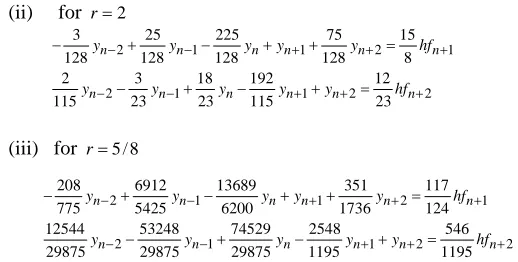
2 , and r = 5/8 into (3.3) and (3.4) gives the coefficients for the first and second point of the BBDF method. These values of r are considered to ensure zero stability and computational efficiency. (i) for r=1

2 1 1 2 1

1 3 9 3 6

10 5 5 10 5

3 16 36 48 12

n n n n n n

y ₋ y ₋ y y ₊ y ₊ hf ₊

− + − + + =

− + − + =

(ii) for r=2

2 1 1 2 1

2 1 1 2 2

3 25 225 75 15

128 128 128 128 8

2 3 18 192 12

115 23 23 115 23

n n n n n n

y y y y y hf

− − + + +

− + − + + =

− + − + =

(iii) for r=5 / 8

2 1 1 2 1

2 1 1 2 2

208 6912 13689 351 117

775 5425 6200 1736 124

12544 53248 74529 2548 546

29875 29875 29875 1195 1195

n n n n n n

y y y y y hf

− − + + +

− + − + + =

− + − + =

Note that the above formula is in the similar form of a standard BDF. This allows us to store the coefficients of the y values and thus avoiding calculating the differentiation coefficients at each step but robust enough to allow for step size variation.

IV. STABILITYOFTHEBBDFMETHODS

In this section, the stability properties of the proposed methods are analyzed to demonstrate their relevance in solving stiff problems. For the method to be of practical importance in solving stiff problems, it must posses at least almost A-stable property.

Definition: A numerical method is called A-stable if the whole of the left half plane,

{

z: Re

( )

z ≤0

}

is contained in the region

( )

{

z R z: ≤1

}

where R z

( )

is called the stability polynomial of the method.

The linear stability properties of the methods are determined through application of the standard linear test problem

y′ =λy, λ<0, λ complex. (4.1) The boundary of the stability region is given by the set of points determined by t=eiθ, 0≤ ≤θ 2π . for which t <1. Below we present the stability region R which corresponds to the 2- point BBDF method drawn in the hλ plane

r = 1 r = 2 stable

stable stable

unstable

stable stable

unstable

(3)

r = 5/8

The stability region which corresponds to the 2-point BBDF method lies outside the close region. From the plot, the BBDF method when r = 2 is A-stable, r = 1 and r = 5/8 is almost

A-stable. Hence, the method derived is suitable for solving stiff ODEs

V. IMPLEMENTATIONOF2-POINTBBDFMETHOD In this section, the application of a Newton-type scheme for obtaining the calculation of y_n₊₁, yn+2 to some stiff equations are described. The 2-point BBDF method can be written in general form as

1 1 2 1 1 1

2 2 1 2 2 2

n n n

y y hf

θ α ψ

+ + +

= + + ⎫

⎬

= + + _⎭ (5.1)

with ψ₁ and ψ₂ are the backvalues.

Equation (5.1) in matrix-vector form is equivalent to

(

I−A Y

)

_n_{+ +}_1,_n ₂ =hBF_n_{+ +}_1,_n ₂+ξ_n_{+ +}_1,_n ₂ with

1 0 0 1

I = ⎢⎡ ⎤_⎥

⎣ ⎦,

1 1, 2

2 n

n n

n

y Y

y

+ + +

+

⎡ ⎤

= ⎢ ⎥

⎣ ⎦,

1

2 0

0

A= ⎢⎡_θ θ ⎤_⎥

⎣ ⎦,

1

2 0 0

B= ⎢⎡α _α ⎤_⎥

⎣ ⎦,

1 1, 2

2 n

n n

n

f F

f

+ + +

+

⎡ ⎤

= ⎢ ⎥

⎣ ⎦ and

1 1, 2

2

n n

ψ ξ

ψ

+ + = ⎢ ⎥⎡ ⎤

⎣ ⎦.

Let

(

)

1, 2 1, 2 1, 2 1, 2

ˆ ₀

n n n n n n n n

F _{+ +} = I−A Y _{+ +} −hBF_{+ +} −ξ _{+ +} = (5.2) To approximate this solution, select Y_n( )i_{+ +}_1,_n ₂ and generate

( )1 1, 2 i

n n

Y _{+ +}+ by applying Newton’s Iteration to the system (5.2) to obtain

( ) ( )

( ) ( ) ( ) ( ) ( )

1

1, 2 1, 2

1

1, 2

1, 2 1, 2 1, 2

i i

n n n n

i i i

n n

n n n n n n

Y Y

F

I A hB Y I A Y hBF Y

Y ξ

+

+ + + +

−

+ +

+ + + + + +

− =

⎡ ∂ ⎛ ⎞⎤ ⎛ ⎞

−⎢ − − _{∂ ⎝}⎜ ⎟_⎠⎥ − − ⎜_⎝ ⎟_⎠−

⎣ ⎦

where J_n _1,_n ₂ F Y_n( )i_1,_n ₂ Y

+ + + +

⎛∂ ⎞_⎛ _⎞

= ⎜_∂ ⎟⎜_⎝ ⎟_⎠

⎝ ⎠ is the Jacobian matrix of

F

with respect to Y .

Choosing the step size

Step size adjustment for 2-Point BBDF is as been stated earlier. On any given step, the user will provide an error tolerance limit, TOL. In the BBDF code, the values of x_n₊₁,x_n₊₂ and

1, 2

n n

y ₊ y ₊ are accepted if the local truncation error, LTE is less than tolerance limit. The LTE is obtained by taking

LTE = y(_n₊p₂+1)−y_n( )₊p₂

where y_n(p₊₂+1) is the (p+1)th order method and y( )_n₊p₂ is the pth order method. If the error estimate is greater than the accepted tolerance limit, the value of y_n₊₁,y_n₊₂ are rejected, then the step is repeated with halving the current step size. In this case, the step ratio r is 2 . After a successful step, the step size increment is given by

1

TOL LTE

p

new old

h = ×c h ×⎜⎛ ⎞_⎟

⎝ ⎠ and if

1.6

new old

h > ×h then h_new=1.6×h_old

where c is the safety factor, p is the order of the method and old

h is the step size from previous block. In our case, c is 0.8.

VI. RESULTS

We tested the performance of the 2-point BBDF method on a set of stiff problems. The problems were solved with tolerances 10−2,10−4 and 10−6 . We will compare the numerical results obtained using 2-point BBDF method with the variable step variable order BDF method which is referred as NBDF. See Suleiman [11] for the details of the algorithm. Below are four of the problems tested.

Problem 1: y x′

( )

=λ

(

y−x

)

+1, 0≤ ≤x 10, y

( )

0 =1 with solution y x

( )

=eλx+x, Eigenvalues:λ= −20, 30, 100− − , Source: Gear, [4].

Problem 2: −1000y+3000−2000e−x, 0≤ ≤x 20, y

( )

0 =0 with solution 3 0.998− e−1000x−2.002e−x.

Problem 3: 1 1 2

2 1 2

998 1998 999 1999

y y y

′ = +

′ = − − ,

( )

1

2 0 1

0 0 y y

=

= , 0≤ ≤x 20

with solution

( )

1000 1

1000 2

2 x x

x x

y x e e

y x e e

− −

= −

= − + . Eigenvalues: λ1= −1,λ2= −1000

Source: Gear, [4]. unstable

(4)

Problem 4:

(

)

2

1 1 2

2 1 2 2

1002 1000

1

y y y

y y y y

′ = − + ′ = − + ,

( )

1 2 0 1 0 1 y y =

= , 0≤ ≤x 20 with solution 1

( )

2 , 2

( )

x x

y x =e− y x =e− Source: Kaps, [6].

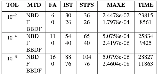
The notations used in the tables take the following meaning: STPS : the total number of steps

TOL : the upper bound for the local error estimate FA : the total number of rejected steps (due to

convergence failure or local error control) IST : the total number of accepted steps MAXE : maximum error

NBDF : implementation of nonblock variable step variable order BDF

BBDF : implementation of variable step 2-point BBDF method

TIME : the execution time in microseconds

Table 6.1(a): Numerical result for Problem 1 for λ= −30

TOL MTD FA IST STPS MAXE TIME

2

10− NBD F BBDF 7 0 32 25 39 25 4.7188e-02 1.2017e-04 16075 8287 4

10− NBD F BBDF 11 0 53 39 64 39 9.0525e-04 2.0600e-06 25919 9275 6

10− NBD F BBDF 16 0 89 74 105 74 1.3568e-05 2.5285e-08 28715 11655

Table 6.1(b): Numerical result for Problem 1 for λ= −50

TOL MTD FA IST STPS MAXE TIME

2

10− NBD F BBDF 6 0 30 26 36 26 5.4862e-0 2 2.3300e-0 4 23214 8571 4

10− NBD F BDF 10 0 53 39 63 39 6.1625e-0 4 2.8412e-0 6 25435 9311 6

10− NBD F BDF 14 0 88 75 102 75 7.9504e-0 6 1.9296e-0 8 27589 11749

Table 6.1(c): Numerical result for Problem 1 for λ= −100

TOL MTD FA IST STPS MAXE TIME

2

10− NBD F BBDF 6 0 30 26 36 26 2.4478e-02 1.7978e-04 23815 8561 4

10− NBD F BBDF 11 0 54 40 65 40 5.0758e-04 2.4197e-06 25834 9425 6

[image:4.612.305.571.49.179.2]

10− NBD F BBDF 16 0 88 76 104 76 5.0793e-06 2.4604e-08 28827 11863

Table 6.2: Numerical result for Problem 2

2

10− NBD F BBDF 5 0 36 30 41 30 5.38298e-03 1.98645e-04 16643 9695 4

10− NBD F BBDF 8 0 74 51 82 51 1.97582e-04 2.64614e-06 21167 11168 6

10− NBD F BBDF 12 0 130 109 142 109 5.42660e-06 1.00448e-06 25460 15459

2

10− NBD F BBDF 13 0 58 31 71 31 3.5277e-01 2.5644e-04 17475 12567 4

10− NBD F BBDF 18 0 101 53 119 53 1.1269e-03 2.5308e-06 22692 16326 6

10− NBD F BDF 22 0 165 122 660 122 6.8001e-06 2.9400e-08 30318 24694

TOL MTD FA IST STPS MAXE TIME

2

10− NBD F BBDF 8 0 48 27 56 27 1.3084e-01 1.0739e-04 23062 11547 4

10− NBD F BBDF 17 0 84 47 101 47 1.1900e-03 5.4820e-06 26540 14243 6

(5)

VII. CONCLUSION

For all the problems tested, numerical results shows that the BBDF methods gives better accuracy with reduction of total steps and lesser computational time.

ACKNOWLEDGMENT

This research was supported by Institute of Mathematical Research, Universiti Putra Malaysia under Fundamental Research Grant Scheme (FRGS) 01-01-07-111FR

REFERENCES

[1] Birta, L.G. and Abou-Rabia, O. (1987), Parallel Block

Predictor Corrector Methods for ODEs, IEEE

Transactions on Computers, c-36(3):299-311.

[2] Cheney, W. and Kincaid, D. (1999), Numerical Mathematics and Computing. Brooks/Cole Publishing Company.

[3] Chu, M. & Hamilton, H. (1987), Parallel solution of ODEs by multi-block methods, SIAM J. Sci. Statist. Comput., 8, pp. 342-353.

[4] Gear, C.W. (1971), Numerical Initial Value Problems in Ordinary Differential Equations, New Jersey: Prentice Hall, Inc.

[5] Houwen, P.J. & Sommeijer, B.P. (1989), Block Runge-Kutta methods on parallel computers, Report NM-R8906, Centre for Mathematics and Computer Science, Amsterdam.

[6] Kaps, P. and Wanner, G. 1981. A Study of Rosenbrock-type methods of high order. Numer. Math.,

38:279-298.

[7] Lambert, J.D. (1993), Numerical methods for Ordinary Differential Equations: The Initial Value Problems, John Wiley & Sons.

[8] Majid, Z. (2004) Parallel Block Methods For Solving Ordinary Differential Equations, PhD Thesis, Universiti Putra Malaysia.

[9] Omar, Z.B. (1999), Developing Parallel Block Methods for Solving Higher Order ODEs Directly, PhD Thesis, Universiti Putra Malaysia.

[10]Shampine, L.F. and Watts, H.A. (1969), Block Implicit One-Step Methods, Math. Comp. 23:731-740.

[11]Suleiman, M.B. (1979), Generalised Multistep Adams and Backward Differentiation Methods for the Solution of Stiff and Non-stiff Ordinary Differential Equations, PhD Thesis, University of Manchester.

[12]Voss, D. and Abbas, S. (1997), Block Predictor-Corrector Schemes for the Parallel Solution of ODEs, Comp. Math.Applic. 33,65-72.