NBER WORKING PAPER SERIES
IS DEBT RELIEF EFFICIENT? Serkan Arslanalp
Peter Blair Henry Working Paper 10217
http://www.nber.org/papers/w10217
NATIONAL BUREAU OF ECONOMIC RESEARCH 1050 Massachusetts Avenue
Cambridge, MA 02138 January 2004
We thank Jeremy Bulow, Steve Buser, Sandy Darity, Darrell Duffie, Nick Hope, Willene Johnson, Paul Romer, Jim Van Horne, Jeff Zwiebel and seminar participants at the AEA Pipeline Project, Columbia, The IMF, Stanford, and The US Department of State for helpful comments. Rania A. Eltom provided excellent research assistance. Henry gratefully acknowledges financial support from an NSF CAREER Award, the Stanford Institute for Economic Policy Research (SIEPR), and the Stanford Center for International Development (SCID). The views expressed herein are those of the authors and not necessarily those of the National Bureau of Economic Research.
©2003 by Serkan Arslanalp and Peter Blair Henry. All rights reserved. Short sections of text, not to exceed two paragraphs, may be quoted without explicit permission provided that full credit, including © notice, is given to the source.
Is Debt Relief Efficient?
Serkan Arslanalp and Peter Blair Henry NBER Working Paper No. 10217 January 2004
JEL No. F3, F4, E6
ABSTRACT
When Less Developed Countries (LDCs) announce debt relief agreements under the Brady Plan, their stock markets appreciate by an average of 60 percent in real dollar terms – a $42 billion increase in shareholder value. In contrast, there is no significant stock market increase for a control group of LDCs that do not sign Brady agreements. The results persist after controlling for IMF programs, trade liberalizations, capital account liberalizations, and privatization programs. The stock market appreciations successfully forecast higher future net resource transfers, investment and growth. Creditors also benefit from the Brady Plan. Controlling for other factors, stock prices of US commercial banks with significant LDC loan exposure rise by 35 percent – a $13 billion increase in shareholder value. The results suggest that debt relief can generate large efficiency gains when the borrower suffers from debt overhang.
Serkan Arslanalp Stanford University Department of Economics Stanford, CA 94305-6072 [email protected] Peter Blair Henry Stanford University
Graduate School of Business Littlefield 277
Stanford, CA 94305-5015 and NBER
Introduction
Bono and Jesse Helms want debt relief for the world’s less-developed countries (LDCs). The Pope and 17 million people are behind them. At a June 1999 meeting of G8 leaders in Cologne, Germany the lead singer of the rock band U2 presented Chancellor Gerhard Schroeder with 17 million signatures in support of the Jubilee 2000 Debt Relief Initiative. In November 1998, Pope John Paul II issued a Papal Bull calling on the wealthy nations to relieve the debts of developing nations in order to “remove the shadow of death.”
Opponents of debt relief occupy less hallowed ground but are no less zealous about their cause, citing at least two reasons why the debt relief campaign is misguided. First, debt relief alone cannot solve the problem of third-world debt. Even if all debt were forgiven, it will accumulate again if income does not grow faster than expenditure (O’Neill, 2002). Second, debt relief can create perverse incentives for debtor countries. By relaxing budget constraints, debt relief may permit governments to prolong wasteful economic policies (Easterly, 2001a).
Do the benefits of debt relief outweigh the costs? Or is it a welfare-reducing market intervention? The stock market provides a natural place to search for answers. Changes in stock prices reflect both revised expectations about future corporate profits and the discount rate at which those profits are capitalized. Consequently, the stock market response to the announcement of a debt relief program collapses the entire expected future stream of debt relief costs and benefits into a single summary statistic: the expected net benefit (current and future) of the program.
The effect of debt relief on the stock market depends on the model of sovereign lending to which one subscribes. Models emphasizing costs suggest three channels through which debt relief may adversely affect the recipient country’s stock market. First, if debt relief allows a
government to persist with wasteful policies, economic growth and corporate profits may be reduced impacting stock prices adversely. Second, countries that do not honor their debts may incur costs in the form of trade sanctions, which may also hurt growth and profits (Bulow and Rogoff, 1989a). Third, debt relief may damage the debtor’s reputation for repayment and raise its future cost of borrowing in international capital markets (Eaton and Gersovitz, 1981).
But, the reputation argument is valid only under assumptions that may not be plausible for LDCs (Bulow and Rogoff, 1989b). Furthermore, both borrower and lenders can benefit from debt relief when the borrower suffers from debt overhang. If each creditor would agree to forgive some of its claims, then the debtor would be better able to service the debt owed to each creditor. Consequently, the expected value of all creditors’ claims would rise (Krugman, 1988; Sachs, 1989). Forgiveness will not happen without coordination, however, because any individual creditor would prefer to have a free ride, maintaining the full value of its claims while others write off some debt.
By forcing all creditors to accept some losses, debt relief can solve the collective action problem and pave the way for profitable new lending (Cline, 1995). By relaxing the intertemporal budget constraint, the new capital inflow may reduce the discount rate in the debtor country. To the extent that the country suffers from a “debt overhang” caused by the collective action problem, debt relief increases the incentive to undertake efficient investments. In turn, these investments may raise expected future growth rates and cash flows (Froot, Scharfstein, and Stein, 1989; Krugman, 1989; Myers, 1977; Sachs, 1989).
On March 10, 1989, the Secretary of the Treasury of the United States, Nicholas F. Brady, called for LDC debt relief. Between 1989 and 1995, sixteen LDCs reached debt relief agreements under the Brady Plan. Figure 1 shows what happened. In the 12-month period
preceding the official announcement of its Brady deal, the average country’s stock market appreciated by 60 percent in anticipation of the event. Stated in dollar terms, the market capitalization of debtor country stock markets rose by a total of 42 billion dollars.
Nor were the wealth gains from debt relief simply a wealth transfer to the debtor nations from western commercial banks. Figure 2 shows that the stock prices of the 11 major U.S. commercial banks with large LDC loan exposure increased by an average of 35 percent—a 13.3 billion dollar increase in market capitalization. Adding the LDCs’ wealth increase to that of the banks gives a rough sense of the Brady Plan’s net benefit to society: 55.3 billion dollars.
To be sure, changes in stock market capitalization measure efficiency gains in a very narrow sense. The stock market welfare metric tells us only whether the benefits to shareholders outstrip any costs involved. In that narrow sense, the results suggest that debt relief may generate ex-post efficiency gains. Of course, debt relief may also induce ex-ante contracting inefficiencies (Shleifer, 2003).1 Our analysis provides no evidence on the size of any such costs, but it is nevertheless important to understand whether debt relief generates ex-post efficiency gains. To the extent that debt restructurings induce ex-ante efficiency losses, the existence of some ex-post efficiency gains is a necessary condition for debt relief to be welfare improving.
In addition to the narrowness of our welfare metric, there are many other reasons to be concerned about using the stock market to evaluate debt relief. One should not look at debtor-country stock market responses in isolation. If the Brady Plan coincides with a positive global economic shock that is unrelated to debt relief, then debtor-country stock markets will rise in concert with stock markets in countries that do not sign debt relief agreements.
In order to distinguish the effect of debt relief from that of a common shock, we compare
1
There is, however, an alternative view. The ex-ante knowledge that debts may have to be restructured could raise efficiency by forcing lenders to be more careful (Darity and Horn, 1988; Fischer, 1987; Bolton and Skeel, 2003).
the stock market response of the Brady countries with the market response of a similar group of countries that did not sign Brady deals. Figure 1 shows that a control group of non-signing LDCs does not experience a significant increase in stock prices. Similarly, Figure 2 shows that the price increase for U.S. commercial banks is not driven by a common shock; there is no significant price increase for a control group of U.S. commercial banks that did not have significant LDC exposure.
Perhaps a greater concern is that anticipated economic reforms drive the price increase in Figure 1. Countries receive Brady deals in return for committing to World-Bank-IMF-supported reforms that are designed to increase openness and raise productivity. So, it is possible that stock prices go up because debt relief signals future reforms. We attempt to distinguish the effects of debt relief from those of reform by making use of a key historical fact. On October 8, 1985, the Secretary of the Treasury of the United States, James A. Baker III, announced a plan for dealing with the Third World Debt Crisis. The Baker Plan called on the debtor countries to undertake extensive economic reforms—stabilization, trade liberalization, privatization, and greater openness to foreign direct investment—but deliberately excluded any plans for debt relief. In contrast, the Brady Plan explicitly called for debt relief in addition to the continuation of the reforms begun under the Baker Plan four years earlier.
The difference in focus of the two plans implies that the “news” in the Baker announcement was the official U.S. push for economic reforms while the “news” in the Brady announcement was the official U.S. push for debt relief. In other words, because economic reforms were enacted under the Baker Plan, their effects should already have been incorporated into stock prices when the subsequent Brady Plan was announced. If markets are efficient, then the market reaction to the Brady Plan should principally reflect the anticipated effect of debt
relief.
The Baker Plan notwithstanding, it is still important to confirm that markets were not surprised by the economic reforms enacted around the time of the Brady Plan. Sections IV and V do just that, and address other concerns about the robustness of our results as well. There, instead of simply inferring that the Brady agreement did not signal any new information about economic reforms, we confront the issue directly. We do so by documenting the dates on which major reforms occurred and testing empirically whether the reforms had any effect on stock prices. While our tests are not definitive, the stock market increase associated with debt relief remains economically large and statistically significant in all regression specifications that include the economic reform variables.
After grappling with concerns about robustness, Section V turns to more primitive issues of interpretation: Why do stock prices rise? Is this a spurious result? Or, does the stock market rationally forecast future changes in the fundamentals? If market values rise because debt relief paves the way for profitable new lending, then the stock market responses should have some predictive power for future changes in net resource transfers (NRTs). Similarly, if the Brady Plan alleviated debt overhang we should see more investment and growth. The descriptive evidence we provide is not definitive, but the stock market responses do help to predict changes in the NRT, investment, and GDP growth for up to five years following the agreements.
I. The Debt Crisis and The Brady Plan
Commercial bank lending to the LDCs surged in the early 1970s. There is no simple way to tell when the loans became non-performing, but a few salient events sent important signals that the quality of the loans was deteriorating. The Mexican default on August 12, 1982
triggered the beginning of the Third-World Debt Crisis. The next five years were marked by frequent debt restructurings and new-money packages that tried, but failed to resolve the crisis (James, 1996, Chapter 12).
A second critical point was reached in February of 1987, when Brazil declared a debt moratorium and suspended all interest payments to its creditors. In response to the Brazilian moratorium, Citicorp announced a $2.5 billion increase in its loan-loss reserves on May 20, 1987. Shortly after Citicorp’s decision, a number of other banks made similar announcements and increased their loan-loss reserves as well (Boehmer and Megginson, 1990). From an accounting perspective, then, May of 1987 appears to be the date when the banks officially recognized that a significant fraction of their LDC loans were non-performing.
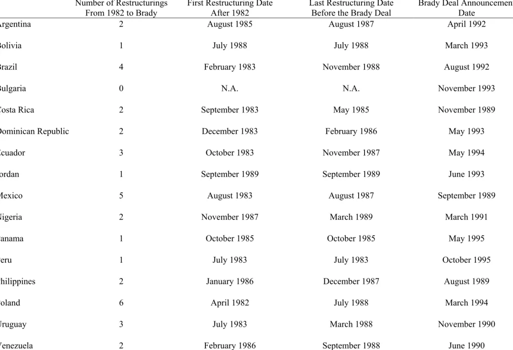
Table I provides a brief summary of the debt restructuring history of the countries that eventually received a Brady Plan: Argentina, Bolivia, Brazil, Bulgaria, Costa Rica, the Dominican Republic, Ecuador, Jordan, Mexico, Nigeria, Panama, Peru, the Philippines, Poland, Uruguay, and Venezuela. Column 2 shows that a large number of restructurings took place in each country between 1982 and the time of its Brady deal. The sheer number of restructurings lends credence to the view that these countries were suffering from debt overhang. Column 3 indicates that a number of countries began to restructure their debt prior to Citicorp’s increase in loan-loss reserves, suggesting that LDC loans may, in fact, have become non-performing prior to May of 1987. Column 4 gives the date of the last debt restructuring that took place before the announcement of a country’s Brady deal; only 4 countries did not restructure their debt after May of 1987.
Finally, Column 5 of Table I lists the announcement date of each country’s Brady Plan. The principal source of announcement dates is International Debt Reexamined (Cline, 1995,
Table 5.3, p. 234). However, the book does not provide announcement dates for Bolivia, Nigeria, Panama, Peru and the Philippines2. For these five countries we retrieved announcement dates using the Lexis-Nexis Academic Universe (http://web.lexis-nexis.com/universe).3 We verified the accuracy of the search by matching the dates obtained from Lexis-Nexis with those in the Quarterly Economic Reports of the Economist Intelligence Unit (EIU).
IA. What Was Restructured?
The goal of the Brady Plan was to restructure the commercial banks’ loans in such a way that interest payments would be reduced, principal forgiven and maturities lengthened. The plan restructured both the public and publicly guaranteed debt claims of the commercial banks.4 The public debt consisted of commercial banks’ loans to the central government. The publicly-guaranteed debt consisted of loans that were publicly-guaranteed by the central government: trade credit; project finance; and bank loans to regional governments and state-owned enterprises (SOEs). Table II shows that the majority of the loans were denominated in dollars, reflecting that most of the debt was held by U.S. Money-Center banks.
Under the Brady Plan, the commercial banks were presented with four options for restructuring the debt:
(1) Discount Bonds: Issue bonds with the total face value of the debt reduced by 30 to 35 percent and an interest rate of LIBOR plus 13/16; a “bullet” single payment maturity of 30 years with US Treasury zero-coupon bond collateral on principal and a rolling guarantee of 12 to 18 months of interest.
2
Cline (1995) provides only the year of the announcement for the Philippines and only the implementation date for Nigeria and Bolivia. It does not provide any dates for Panama and Peru because these countries were still
negotiating their debt relief agreements at the time of the book’s publication. 3
A data appendix containing the complete list of articles that were uncovered by the Lexis Nexis search is available upon request.
4
It is possible that minor amounts of market issues such as bonds or notes were also restructured, but we could not find any evidence on such restructurings.
(2) Par Bonds: Issue bonds worth the full face value of the debt with an interest rate of 6 percent and similar maturity and collateralization as the discount bonds. (3) New Money: Retain the full value of the debt, but issue new loans in the amount of 25 percent of current exposure over the next three years with at least half of the new money coming within the first year.
(4) Cash Buybacks: Repurchase of the debt at a specific price.
The options chosen by the banks varied by country. In countries that were lightly indebted, banks favored the new money option, whereas in heavily indebted countries there was very little new money. Cash buybacks were limited to small, low-income countries with little bank debt such as Costa Rica. The discount bond was designed for banks concerned about limiting the risk of interest rate fluctuations. The par bond was intended for banks located in countries where regulatory and tax considerations made maintaining full face value preferable (Cline, 1995).
In return for accepting the four-point restructuring menu, the banks received 25 billion dollars of enhancements—collateral for principal and a rolling fund to cover several interest payments—in the form of U.S. Treasury Bonds (Cline, 1995, Chapter 5). The debtor countries paid for the Treasury securities with loans from the International Monetary Fund (IMF) and the World Bank. Although they needed a member-country-financed capital injection to make these loans, it is important to remember that the Fund and the Bank "…lent at rates that reflect at least opportunity cost of Treasury bonds...so that the public sector is not providing concessional financing. The short answer, then, is that the public-sector enhancements did not cost anything." (Cline, 1995, p. 265). Of course there may have been transaction costs, but they were probably nothing more than rounding error relative to the overall sums of money involved.5
Table III demonstrates that roughly 202.8 billion dollars worth of debt was restructured,
5
The Treasury, the IMF and the Bank can be seen as the agents that were necessary for overcoming the transaction costs that stood in the way of the commercial banks negotiating a Coasian (1960) solution to the debt problem.
resulting in 64.7 billion dollars of debt relief. The average spread fell from 17/16 over LIBOR on the loans before the Brady Plan to 13/16 over LIBOR on the discount bonds after the restructuring.6 Similarly, debt prices rose. In the year prior to restructuring, the average country’s debt was trading at 32 cents on the dollar in the secondary market. In the month of the Brady Deal, the average price rose to 42 cents on the dollar. Finally, the average maturity of the debt increased from 15 to 30 years.
II. Data and Descriptive Findings
The principal source of stock market data is the IFC’s Emerging Markets Data Base (EMDB).7 Stock price indices for individual countries are the dividend-inclusive, U.S. dollar-denominated and local currency-dollar-denominated IFC Global Indices. For most countries, EMDB’s coverage begins in December 1975, but for others coverage begins in December 1984. Each country’s U.S. dollar-denominated stock price index is deflated by the U.S. consumer price index (CPI), which comes from the IMF’s International Financial Statistics (IFS). The local currency-denominated index is deflated by the local consumer price index for each country, which is also obtained from the IFS. Returns and inflation are calculated as the first difference of the natural logarithm of the real stock price and CPI, respectively. All of the data are monthly.
Reliable stock market data exist for only 10 of the Brady countries: Argentina, Brazil, Ecuador, Jordan, Mexico, Nigeria, Peru, the Philippines, Poland, and Venezuela. We bring Bolivia, Bulgaria, Costa Rica, Dominican Republic, Panama, and Uruguay back into the picture in Section VI where the focus of analysis moves from financial to real data.
6
For an early analysis of LDC loan spreads see Edwards (1984). 7
IIA. Selection of the Control group
The control group consists of all developing countries that: (1) Did not receive a Brady plan; and (2) Have stock market data in the International Finance Corporation (IFC) Emerging Market Data Base. There are 16 such countries: Chile, China, Colombia, the Czech Republic, Greece, Hungary, India, Indonesia, Korea, Malaysia, Pakistan, South Africa, Sri Lanka, Thailand, Turkey, and Zimbabwe.
It is important to ask whether the selection of the control group introduces statistical bias. The purpose of the control group is to determine whether the stock price increase in the debtor countries was driven by a global economic shock unrelated to debt relief. Therefore, it is crucial that the control group not consist of countries in such an abject state of development that their stock markets would not respond to a positive external shock, no matter how favorable. We address this concern by examining the characteristics of the Brady and control groups in some detail.
The Brady countries and the control group display similar geographical dispersion. Both groups contain countries from Latin America, Asia, Africa, and Eastern Europe. One significant difference is that Latin American countries comprise the largest fraction of the Brady countries while the control group primarily consists of countries in Asia. History suggests that the relatively heavier weighting of Asian countries in the control group will make that group the stronger economic performer. We confirm this suspicion by comparing the Brady countries and the control group using two standard measures of economic performance, growth and inflation.
The control group outperforms the Brady countries on both measures. Between 1980 and 1999 the median growth rate of per capita GDP for the control group was 3 percent. The Brady group grew by only 1 percent per year during the same time period. GDP growth was also less
volatile in the control group. The standard error of GDP growth for the control group was 1 percent, as compared to 2 percent for the Brady group. Finally, the control group has a lower and less volatile rate of inflation: a median of 11 percent and a standard deviation of 3 percent. The corresponding numbers for the Brady countries are 27 and 18.
To summarize, the median country in the control group has faster and less volatile growth together with lower and less volatile inflation than its Brady group counterpart. To the extent that superior long-run economic performance is positively correlated with better-managed economies, we would expect stock markets in the median control-group country to be more responsive to any auspicious common shock.
Finally, analyzing the universe of countries that received Brady Deals does not introduce any obvious selection bias. True, the countries that enter into Brady Deals are probably the ones that are most likely to benefit from debt relief. But that is precisely the point. We are not trying to estimate the average effect of debt relief on a randomly selected country. Just as it does not make sense to try to measure the effect of a medical treatment on a healthy individual, neither is it sensible to estimate the effect of debt relief on a country where debt overhang is not an issue.
IIB. Descriptive Findings
This subsection presents descriptive evidence on how the stock market responds to news of a future debt relief agreement. For each Brady country we calculate the average monthly stock return over the entire sample. The average monthly return is a proxy for the expected monthly return. Subtracting a country’s expected return from its actual return gives the abnormal return.8
8
Let month [0] be the month in which a Brady debt relief announcement takes place for a given country. Similarly, let [-12] denote the 12th month before the debt relief announcement, so that [-12, 0] denotes the one-year window preceding the announcement. The cumulative abnormal return for a country is defined as the sum of its abnormal returns from month –12 to month 0.
Figure 1 plots the average cumulative abnormal return across all ten Brady countries in event time. The average Brady country stock market experiences cumulative abnormal returns of 60 percent in real dollar terms. In other words, the real dollar value of the stock market increases by 60 percent more than it does in a typical year. Now look at the graph for the control group. If a common shock caused stock prices to go up in the Brady countries, then we should also see an increase in the stock prices of the control group. This is not the case. The average cumulative abnormal return for the control group is close to 0.9 The preliminary conclusion is that the stock price increase in the debtor countries is not due exclusively to a common shock that has favorable effects on all emerging stock markets.
Since there are only ten countries in the Brady stock market group, one country may dominate the results. To explore this possibility we conduct median tests in the following way. For each of the ten countries we compute the median annual stock return. The stock return in the 12-month period preceding the Brady announcement exceeds the median, annual return for every country except Peru. We also conducted median tests in local currency, and the results were the
9
For a given Brady country, the control group abnormal returns are calculated as follows. Fix the announcement date [0] for the country in question. Next, for each of the 16 countries in the control group, calculate the abnormal returns for [-12, 0]. This calculation gives 16 sets of abnormal returns for the fixed Brady-country date. Next, calculate the average of these 16 sets of abnormal returns and you have the single series of abnormal returns for the control group associated with the first country. Now repeat the procedure for the other 9 Brady countries. Doing so yields 10 series of average abnormal returns for the months [-12, 0]. Finally, taking the average across all 10 series gives the average abnormal return for the entire Control group.
same. Peru is the only country whose stock return during the 12-month announcement window was less than its median 12-month return.
Another concern is that the results may be sensitive to whether real returns are measured in dollars or the local currency. To address this concern, we replicated Figure 1 using real local currency returns instead of real dollar returns. The resulting graph was virtually identical to Figure 1. Since the choice of currency makes little difference, the formal empirical analysis in Section IV focuses on the dollar-denominated returns.
By constructing a control group of relatively strong economic performers, we are able to distinguish the effect of the Brady Plan from that of a common shock. But constructing the control group in this way raises the question of whether we have properly addressed the counterfactual: Would stock prices have gone up in the Brady Countries had they not received debt relief?
Addressing the counterfactual requires constructing a control group that bears a greater resemblance to the Brady countries. To do so, we replicated our experiment using two alternative control groups. The first consisted of the highly or moderately indebted countries of the original control group: Indonesia, Pakistan, Colombia, Malaysia, and Turkey; the second consisted of all the Brady countries that were still waiting to receive their Brady deals. The graphs were almost identical to Figure 1.10 There was no significant increase in the stock market in either of the two alternative control groups in the 12-month period preceding debt relief announcements.
IIC. Why Use A 12-Month Event Window?
10
Using a 12-month window provides a reasonable characterization of the data, because the announcement of a debt relief agreement is less a discrete occurrence than it is a series of events during which the public gradually learns the details of the government’s negotiations to reduce its external debt burden. Table IV illustrates the point for three representative countries: Argentina, Nigeria and Venezuela.
Argentina had a 9-month window of negotiations with its external creditors, extending from July of 1991 to the official announcement of an agreement in April of 1992. In July of 1991, the Economist Intelligence Unit reported, “The International Monetary Fund approves a 1 billion dollar stand-by loan.” On September 20 of 1991, the Financial Times reported “Domingo Cavallo, comes to Washington to jump-start negotiations on the country's $61bn debt.” On March 31, 1992 the Financial Times reported, “Argentina secures a $3.15bn extended facility fund loan from the IMF. Approval of the loan is important for securing a restructuring with the creditor banks.”
Nigeria had a 10-month window of negotiations with its external creditors, extending from May of 1990 to its official announcement in March of 1991. The window of public negotiations began with a Financial Times story on October 3, 1990, “The resolution of the five-month deadlock over rescheduling terms for Nigeria's $5.5bn commercial bank debt appears likely.” The reference to a 5-month deadlock suggests that the sequence of public events may actually have begun as early as May of 1990. Between October 1990 and March of 1991, the
Financial Times ran at least two more stories about Nigeria’s negotiations with its creditors.
Finally, Venezuela had an 11-month window of negotiations that began with the
Washington Post’s declaration on July 25, 1989: “the Mexican deal will set a pattern for dealing
at the head of the list.” On March 21, 1990 the New York Times reported “Venezuela and its creditor banks reach an agreement on the basic terms of a deal.”
The average length of the window in these three countries is 10 months. This estimate is based on the earliest reported news headlines that we could find through Lexis-Nexis. Even if these are, in fact, the earliest public releases of information, the possibility remains that the news was “leaked” to the markets prior to the news dates that we collected. Admittedly, constructing the event window is at least as much art as it is science, but all things considered, a 12-month window does no obvious harm to the data. Furthermore, Section IV estimates results using 12-month, 9-12-month, 6-month and 3-month windows—the effect of debt relief on the stock market is positive and significant in all specifications.
Of course, a long event window raises the specter of reverse causality. Instead of debt relief generating a stock market boom, maybe rising stock markets and improved economic prospects cause countries to write-down their debts? In thinking about this question, it is important to remember that countries cannot simply decide that they want debt relief and make it so. This is because debt relief requires a mutual agreement between parties: The debtor requests a write down and the creditor agrees to forgive some of the debt. Reaching such agreements can take a long time because both the debtor country and the creditor banks want to exercise their bargaining power (Froot, Scharfstein, and Stein, 1989). Consequently, negotiations might reach a deadlock, which could take many months to resolve, as illustrated by the case of Nigeria in October 1990 (Table IV). Given the length of time and the number of parties involved in sovereign debt restructurings, it is difficult to believe that a debtor country would be able to push
through a debt relief agreement as a swift policy response to a rising stock market and improving economic prospects. 11
Four central facts emerge from this section: (1) Stock markets in debtor countries rise by 60 percent in real dollar terms in response to news of debt relief; (2) The response is uniformly positive across debtor countries; (3) The effect is not an artifact of the currency in which the revaluation is measured; (4) The control group never experiences a revaluation of greater than 10 percentage points. Having eliminated outliers, currency concerns, and common shocks as explanations for our result, there is another, much trickier, issue to address before proceeding to formal statistical estimation.
III. Are the Revaluations Driven by Debt Relief or Reforms?
Countries receive debt relief in return for committing to economic reforms (Cline, 1995). These reforms take four principal forms—inflation stabilization, privatization, trade liberalization, capital account liberalization—and there is evidence that the stock market responds favorably to each one of them (Megginson and Netter, 2001; Perotti and Van Oijen, 2001; Henry, 2000a, 2002, 2003). Therefore, a central issue is whether debt relief or economic reforms drive the debtor-country stock price increases. To address the issue we conducted a search to pinpoint the dates on which the reforms occur. The results are outlined in Table V.
The stabilization dates come from the International Monetary Fund’s Annual Reports and Henry (2002). We use the Economist Intelligence Unit’s Quarterly Economic Reports to identify trade liberalization dates. We check the EIU dates against the trade liberalization dates
11
Negotiations during the debt crisis were made less unwieldy by proceeding in two steps. First, a select committee of the largest lenders and the debtor country agreed on the choice of menu options. Second, all of the banks then decided on the term sheet. Although, the two-step process made the negotiations less cumbersome, it also increased the time to reach a final agreement because it required meetings on two separate dates.
in the World Bank publication, Trends in Developing Economies (1994) and those in Sachs and Warner (1995). The privatization dates come from the World Bank Privatization Transaction
Database, which contains the names and dollar amounts of all privatizations occurring between
1988 and 1999. We use the privatization database to identify the first year in which there were recorded sales of state-owned enterprises. Once we know the year of the first sale, we search the EIU’s Quarterly Economic Reports for the month in which the start of the privatization program was announced. We also check the EIU to make sure that there were no privatizations preceding the starting date of the database. Finally, the capital account liberalization dates come from Henry (2003).
A close examination of Table V illustrates the point of the exercise. All of the debtor countries began implementing major economic reforms before the Brady deal and continued to do so after the deal was announced. For example, Column 3 of Table V shows that an official agreement with the IMF immediately precedes, or follows on the heels of every Brady deal. Since IMF programs follow all of the Brady agreements, Brady agreements may drive up stock prices because they signal future IMF agreements. Just as debt relief agreements may signal future IMF agreements, IMF agreements may in turn signal countries’ commitment to future economic reforms (Williamson, 1994; Collins, 1990; Bruno and Easterly, 1996). If debt relief agreements are a signal of future productivity-enhancing reforms, then Figure 1 may erroneously suggest that debt relief drives up valuations when, in fact, the anticipation of future economic reforms is instead responsible.
IIIA. The Baker Plan Versus the Brady Plan
market to reforms from the response of the stock market to debt relief. Our identification strategy hangs on a key historical fact. The Baker Plan called on countries to undertake extensive reforms but deliberately excluded any plans for debt relief.12 In contrast, the Brady Plan called for the continuation of reforms begun under the Baker Plan in 1985, but also made an explicit call for debt relief.
The difference in focus of the two plans implies that the “news” in Baker was the official U.S. push for economic reforms while the “news” in Brady was the official U.S. push for debt relief. In other words, because economic reforms were enacted under the Baker Plan, their effects should already have been incorporated into stock prices when the Brady Plan was announced four years later. If markets are efficient, then the stock price reaction to the Brady Plan should principally reflect the anticipated effect of debt relief.
On October 8, 1985 the Secretary of the United States Treasury, James A. Baker III, unveiled his plan for dealing with the third-world debt crisis at the Annual International Monetary Fund World Bank Meeting in Seoul, Korea. Secretary Baker begins by stressing the importance of macroeconomic stabilization:
If the debt problem is going to be solved there must be a “Program for Sustained Growth”, incorporating… First and foremost, the adoption by principal debtor countries of comprehensive macroeconomic and structural policies, supported by the international financial institutions, to promote growth and balance of payments adjustment, and to reduce inflation (Baker, 1986, p. 308).
After spelling out the need for stabilization Baker called for structural reforms:
For those countries which have implemented reforms to address the imbalances in their economies, a more comprehensive set of policies can now be put in place…We believe that such institutional and structural policies should include: increased reliance on the private sector, and less
12
There were 17 countries included in the Baker Plan: Argentina, Bolivia, Brazil, Chile, Colombia, Costa Rica, Cote d’ Ivoire, Ecuador, Jamaica, Mexico, Morocco, Nigeria, Peru, Philippines, Uruguay, Venezuela, and Yugoslavia. The 16 countries included in the Brady Plan are listed in Table 1.
reliance on government;…tax reform, labor market reform and development of financial markets;…market opening measures to encourage foreign direct investment and capital inflows, as well as to liberalize trade (Baker, 1986, p. 310).
The enumeration of desired reforms in Secretary Baker’s speech displays an attention to detail that underscores the importance of what he does not mention: debt relief. Baker uses or alludes to the word “reform” more than 25 times during the course of his speech. But the phrases “debt relief” and “debt reduction” do not appear.
While testifying before the House Committee on Banking, Finance and Urban Affairs, two weeks later, Secretary Baker erased any doubt that the absence of the phrase “debt relief” from his speech was an error of omission. Witness the interchange between Secretary Baker and Representative Bill McCollum of Florida.
McCollum: “Do you anticipate that there might have to be some forgiveness or moratorium on interest payments to some of these countries in the process by the commercial lending institutions in this country?”
Baker: “No, sir; I don’t contemplate that and I think that would be the wrong road for us to start down. . .I don’t think there should be any moratorium; I don’t think there should be any capitalization of interest proposals or anything like that…” (Baker, 1985, p. 26).
Roughly four years later, on March 10, 1989, Baker’s successor, Nicholas F. Brady revealed his plan for dealing with the debt crisis to the Brookings Institution and the Bretton Woods Committee Conference on Third World Debt. In no uncertain terms, Secretary Brady stated that the U.S. government was going to continue pushing the reforms that began under the Baker Plan:
In 1985 we paused and took stock of our progress in addressing the problem. As a result of that review, together we brought forth a new strategy, centered on economic growth. This still makes sense…The
experience of the past four years demonstrates that the fundamental principles of the current strategy remain sound: Growth is essential to the resolution of debt problems. Debtor nations will not achieve sufficient levels of growth without reform (Brady, 1989, p. 116).
But in addition to the reforms, Secretary Brady explicitly called for debt relief. In sharp contrast to the words of his predecessor in Seoul four years earlier, Brady explicitly used the phrase “debt reduction” or “debt service reduction” eighteen times in his speech. For example:
Let me reiterate that we believe that the fundamental principles of the current [Baker] strategy remain valid. However, we believe that the time has come for all members of the international community to consider… debt and debt service reduction on a voluntary basis…The path toward greater creditworthiness and a return to the markets for many debtor countries needs to involve debt reduction (Brady, 1989, pp. 117-118).
In a rare moment of consensus, U.S. politicians, the international banking fraternity, officials in debtor countries, and academics all agreed that the Brady Plan represented a continuation of the Baker Plan’s commitment to reforms, with the important change that debt relief now had the official support of the United States Treasury.13 James D. Robinson III, Chairman and CEO of American Express best summarizes the consensus in his response to Brady’s speech:
In the next few days we will encounter statements to the effect that the Brady Plan means the death of the Baker Plan. My advice is to ignore these statements. The focus of both plans is on growth in the debtor countries. The principles of the Baker Plan have not been abandoned. They will have to be embodied in the Brady Plan as it is carried forward. What is new, of course, is the explicit recognition of debt reduction as an essential element in the search for solutions (Robinson, 1989, p. 101).
The historical record leaves little ambiguity about the fundamental similarity—reforms— and the key difference—debt relief—between the Baker Plan and the Brady Plan. Nevertheless, there are several potential concerns with our identification strategy. We will enumerate and
13
For example, see the reactions of democratic senators Bill Bradley (1989) and Paul Sarbanes (1989); Former Mexican Finance Minister, Jesús Silva Herzog (1989), and Stanley Fischer (1989)
attempt to address these concerns in Section IV. But, first things first. Before we can interpret the results, we need to know what they are. This is the topic to which we now turn.
IV. Formal Empirical Results
We evaluate the statistical significance of the relationships apparent in Figure 1 by estimating the following regression:
1 2
it i it it it
R =α γ+ BRADY +γ CONTROL +ε , (1) Where R is the real return in dollars on country ’s stock market index in month t, it i BRADY is it
a dummy variable that is equal to one in [-12, 0]. CONTROL is a dummy variable that is equal to one in all of the control countries in Brady-Announcement months [-12, 0]. We also estimate BRADY and CONTROL using nine-month [-9, 0], six-month [-6, 0], and three-month [-3, 0] windows. The country-specific intercepts allow for the possibility that average expected returns may differ across countries due to imperfect capital market integration.
Equation (1) constrains the coefficients on BRADY to be the same across all months, which means that the parameter γ1 measures the average monthly stock market response to all Brady Plan Announcements. Since the dummy variable for the event window is twelve months long, the total stock market response to debt relief for the Brady countries is given by twelve times the parameter estimate.
A different estimation technique would be to use a seemingly unrelated regression (SUR). This approach would have the advantage of providing a unique coefficient estimate for each country for each event. However, there are also disadvantages to this approach. The low power of hypothesis tests in unconstrained systems severely weakens the ability of the event study methodology to detect the impact of the event. Second, SUR requires a balanced panel.
Due to the limited time series availability of stock market data, creating a balanced panel would result in discarding some of the 10 debt relief events. Given data limitations, the pooled cross-section time series framework seems appropriate.
With an unbalanced panel, it is not possible to relax the assumption of no contemporaneous correlation of the error term across countries. Therefore, we will take indirect precautions. Specifically, three of the alternative regression specifications to equation (1) will estimate abnormal returns relative to the World stock market index, US stock market index, and finally IFC’s emerging stock market index. Since all of the sample countries are emerging markets, the inclusion of a composite emerging market index as a right-hand-side variable will partially control for contemporaneously correlated disturbance terms. Including the emerging market index does not change the results.
IVA. Basic Results
The first row of Table VI (Panel A)—labeled ‘Country-Specific Mean’—gives the results from the baseline specification in equation (1). White standard errors are reported in parentheses. Column (1a) shows that the coefficient on BRADY for the 12-month window [-12, 0] is 0.05 and is statistically significant at the 1 percent level. Multiplying the coefficient by 12 gives the total effect, a 60-percent increase in the real dollar value of the stock market. Column (1b) gives the coefficient estimate for the CONTROL dummy. In contrast to the estimate for the BRADY countries, the revaluation effect associated with the control group is economically weak, 0.005, and statistically insignificant. Column (1c) provides the p-value from a two-sided F-test of the hypothesis that the coefficient estimate on BRADY is equal to the coefficient estimate on CONTROL. The p-value for this test is 0.001. The difference between the BRADY
estimate and the CONTROL estimate is statistically significant. In other words, the stock market in BRADY countries rises by roughly 60 percentage points more than it does in the CONTROL group.
The results using 9-month, 6-month, and 3-month windows are all consistent with the 12-month estimates. The coefficient estimate of BRADY ranges from 0.048 to 0.052 and is statistically significant in every specification. Furthermore, the BRADY estimate is always significantly larger than the estimate of CONTROL (except for the 3-month window). Row 2 of Table VI (Panel A)—labeled, ‘Constant Mean’—presents estimates of equation (1) using a constant intercept term, α , instead of country-specific intercept terms. The results are almost identical to those in Row 1.
IVB. Controlling for World Stock Markets
Equation (1) provides a parsimonious baseline specification of abnormal returns, but it does not allow for the influence of world stock markets on local returns. In order to do so, we follow Kho, Lee and Stulz (2000) and use the international capital asset pricing model (ICAPM) to measure the expected return on each country’s stock market index. Specifically, we now estimate:
1 2
W
it i t it it
R =α β+ R +γ BRADY +γ CONTROL+ε , (2) Where R is the real return in dollars on the Morgan Stanley Capital Market Index (MSCI) in tW
month t. While barriers to the international movement of capital may raise questions about the economic assumption of an ICAPM, as a purely statistical matter, returns on world stock market indices do have some predictive power for stock returns in the countries under consideration
(Henry 2000a).14
Row 3 of Table VI (Panel A) presents estimates of BRADY and CONTROL using equation (2). Row 4 presents estimates that use real U.S. stock returns, US
t
R , in place of W t R .
Row 5 presents estimates that use the real dollar return on the IFC Emerging Market index,
LDC t
R , in place of W t
R . Row 6 presents estimates that use all three sets of world stock returns
simultaneously. The results in Rows 3 through 6 perfectly mirror those under the benchmark specification in Rows 1 and 2. The coefficient on BRADY is statistically significant under all four ICAPM specifications. The point estimate ranges from 4.9 to 3.9 percent per month, and the estimate of BRADY is significantly larger than the estimate of CONTROL in all but the 3-month window estimates.
IVC. Other Robustness Checks
The estimates in Panel A of Table VI adjust for cross-country heteroscedasticity and cross-country correlation, but they do not account for potential serial correlation in the error terms. Hence, White standard errors may not be sufficient to ensure the reliability of the estimates in Panel A. To address this concern, Panel B of Table VI re-estimates all of the specifications in Panel A using Feasible Generalized Least Squares (FGLS). FGLS allows for the possibility of serial correlation, in addition to correcting for cross-country heteroscedasticity. The estimations using FGLS in Panel B yield the same conclusions as the OLS estimates in Panel A. Every FGLS point estimate of BRADY in Panel B of Table VI is statistically significant. The FGLS monthly point estimates of BRADY are smaller than those obtained
14
For conceptual discussions of the international capital asset pricing model see Frankel (1994); Stulz (1999a); Tesar (1999); Tesar and Werner (1995); and Tesar and Werner (1998). For empirical evidence on the real effects of increased capital market integration, see Henry (2000b).
using OLS, but they are still large. The smallest point estimate for the 12-month window is 0.034— a total revaluation of greater than 40 percent. Furthermore, the coefficient on BRADY remains significantly larger than the coefficient on CONTROL in all of the specifications except for some of those that use 3-month windows.
V. Alternative Explanations
Section IV establishes the statistical robustness of the central result: In anticipation of the announcement of debt relief agreements, there is an economically large and statistically significant increase in the stock market. There are, however, many possible interpretations of this fact. Section III argues that since markets are forward looking, stock prices in the debtor countries should have priced in the effect of economic reforms at the time of the Baker Plan. If the only “news” in the Brady Plan was the information about debt relief then debt relief may plausibly be viewed as the proximate cause of the revaluation.
Plausibility, however, hangs on the validity of three key assumptions: (1) The market believed that the Baker Plan would lead to reforms; (2) The depth and scope of reforms under Brady were the same as those under Baker; and (3) The reforms went through as expected. Figure 3 leaves little doubt that market participants in debtor countries viewed the Baker Plan as a signal of future economic reforms—stock market values increased by an average of 22 percent in real dollar terms over the 12-month period preceding the Baker Plan.15 So, the two key questions are: Were the depth and scope of the reforms the same under Baker and Brady? And did the reforms go through as anticipated? We now address each of these questions in turn.
15
The countries represented in Figure 3 match the countries represented in Figure 1 almost perfectly. Jordan is the only country represented in Figure 1 that is not represented in Figure 3. This is because Jordan was not a Baker country.
VA. Do Differences in Depth And Scope of Reforms Drive the Results?
If the Brady Plan called for structural changes that were not a part of the Baker Plan, then the Brady Plan could contain important new information about reforms. Therefore, the estimates in Section IV may be interpreted as the marginal effect of debt relief only if the reforms implemented under Baker were not be radically different from those that continued under Brady. Consistent with the earlier quote by American Express CEO James D. Robinson III (see Section IIIA), a careful reading of both Baker and Brady’s speeches reveals no significant differences between the reforms advocated under each plan.16 In fact, the reforms called for by the two plans were so similar that they came to be summarized as the “Washington Consensus” by John Williamson (1990)17. An exhaustive summary of the Washington Consensus is beyond the scope of this paper—see Williamson’s paper for details—but again, the central idea was that countries should stabilize inflation, privatize state-owned enterprises, liberalize trade, and permit greater foreign direct investment.
VB. Did the Reforms Go Through As Anticipated?
There may have been a consensus about the desired set of reforms, but the very need for a Brady Plan in addition to the Baker Plan suggests that at least some of the expected reforms did not go through as planned.18 If the countries did not actually undertake the reforms they agreed to implement under the Baker Plan, then signing a Brady agreement could signal to the markets a
16
See also the remarks by Stanley Fischer (Fischer, 1989 and 1990). 17
See also Fischer’s comments on Williamson’s paper (Fischer, 1990).
18 This is a complicated issue. The Baker Plan called for three things: reforms, financial support from the International Financial Institutions (IFIs), and new money from the commercial banks. The Baker Plan assumed that the banks would be willing to lend new money as long as countries implemented reforms. This assumption turned out to be wrong. In spite of substantial—if not complete—reforms on the part of the debtors, the banks were unwilling to extend new loans. There is a widely held view that the banks were unwilling to do so because of the existing debt overhang (Cline, 1995).
new commitment to reform. Accordingly, the stock price increase in that case would reflect the expected effects of both reforms and debt relief.
If the Brady Plan contained new information about reforms, then a more accurate measure of the effect of debt relief might be the difference between the stock market reaction to the Brady Plan and the reaction to the Baker Plan. The reaction to the Brady Plan measures the effect of debt relief and reforms; the stock market reaction to the Baker Plan measures the effect of reforms only. Thus, in principle, the difference between the Baker revaluation depicted in Figure 3 (22 percentage points) and the Brady revaluation (60 percentage points) yields the marginal effect of debt relief: 38 percentage points.
But viewing the difference in the market’s response to Baker and Brady as the marginal effect of debt relief is also not without problems. The expected effect of reform on the stock market is given by the benefit of reform conditional on success times the probability of success. Even assuming that the conditional benefit of a successful reform was the same under Baker and Brady, there may have been differing probabilities of success. For example, some argue that debt relief gave governments the capital they needed to push through further reforms with a populace that had grown weary with austerity measures and structural adjustment.19 If this is the case, then the difference between the stock market response to Baker and Brady reflects both the effect of debt relief and the higher probability of successful reforms under Brady.
VC. Direct Controls for the Effect of Economic Reforms
We deal directly with the concern that economic reforms implemented around the time of the Brady Plan may still have contained some “news” by including dummy variables for reforms
19
in all of our earlier regressions. There is sufficient heterogeneity in the timing of the economic reforms (Table V) to allow us to control directly for their effect on stock prices. To do so, we construct a series of reform dummies for each country: TRADE; PRIVATIZE; LIBERALIZE. These variables take on the value 1 during the month a reform is announced and in each of the preceding 11 months. We then estimate the following regression:
1 2 3 4 5
W
it i t it it it it it it
R =α β+ R +γ BRADY +γ CONTROL +γ TRADE +γ PRIVATE +γ LIBERALIZE +ε
(3).
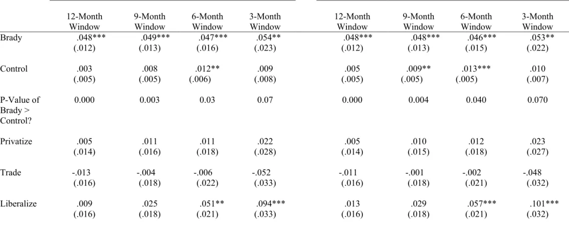
Table VII presents the results. The coefficient on BRADY is significant at the 1 percent or 5 percent level for every window, and is significantly different from the coefficient on
CONTROL in every specification. The results are also consistent with the view that stock prices
incorporated the effect of economic reforms long before the Brady Plan was announced.
Stock market liberalizations are the only economic reform implemented around the time of the Brady Plan that have any effect on the markets. It is no coincidence that stock market liberalizations are also the only reform in our regression that was not a part of the Washington Consensus. The Baker Plan called for the liberalization of foreign direct investment; liberalization of portfolio equity investment is not directly mentioned. In other words, stock market liberalizations were a surprise. Consistent with a number of papers, the stock market liberalization dummy is significant for the [-6, 0] and [-3, -1] windows (Henry, 2000a, b, 2003).
Because every debt relief agreement closely coincides with an IMF agreement, we cannot disentangle the debt relief effect by inserting into equation (3) a dummy variable for IMF programs that coincide with debt relief announcements. An IMF dummy constructed in that way would be collinear with the BRADY dummy and present the attendant econometric problems. Therefore, we adopt a different tack. We examine whether the stock market responds to IMF agreements that are not accompanied by debt relief.
We do so by constructing for each country a list of all IMF programs that did not occur within a year (before or after) of the announcement of its Brady agreement. We then create a dummy variable, IMFPROGRAM, which takes on the value one for all such programs, and estimate the following regression:
1
W
it t it it
R = +α βR +γ IMFPROGRAM +ε . (4) Following the earlier specifications, we estimate 12-month, 9-month, 6-month, and 3-month windows. If the stock market responds positively to IMF agreements that are not accompanied by debt relief, then the estimate of γ1 should be positive and significant.
There is no evidence that the stock market responds positively to IMF agreements that are not associated with a Brady debt relief agreement. The coefficient estimate of IMFPROGRAM is negative and statistically insignificant in every specification. The estimate for the 12-month window is –0.016; the estimate for the 9-month window is -0.011; the estimate for the 6-month window is -0.004; the estimate for the 3-month window is -0.027.20
VI. Why Do Market Values Rise?
Do the debtor country stock price increases reflect an irrational exuberance about the efficacy of debt relief? Or, do they rationally forecast important subsequent changes in the countries’ economic fundamentals? Theory points to three pieces of data that can help answer the question: the net resource transfer (NRT), investment, and growth.
The NRT is the net flow of real resources into a country. In theory, LDCs should experience positive NRTs, as the rate of return in these countries should be higher than in rich
20
The insignificance of the IMFPROGRAM variable is consistent with evidence that the market responds positively to IMF agreements, only when they are announced in the midst of high inflation (Henry, 2002).
countries. However, the NRT may suddenly turn negative if adverse shocks or poor economic management: (1) drive creditors to call in existing loans; and (2) make potential new creditors unwilling to lend.
Because the government pays its external debt by taxing domestic firms and households, the private sector’s expected future tax burden increases sharply when the country’s NRT suddenly turns negative. The higher future tax burden discourages investment and results in creditors being able to recover less than they would if some of the debt was forgiven. By reducing the implicit marginal tax rate on expected future cash flows, debt relief can remove the debt overhang, thereby restoring positive NRTs, investment, and growth (Krugman, 1989; Sachs, 1989).
VIA. Is There a Change in NRT, Investment, and Growth?
Table VIII reveals a clear association between the Brady debt restructuring and changes in the sign of the NRT. In every one of the years from [-18, -9] the median NRT to the Brady countries is positive. At the onset of the Debt Crisis (roughly year –7), the NRT turns negative and remains so until the Brady Plan (year 0). After the Brady Plan, the NRT turns positive and remains so for the rest of the sample. The table also shows that the change in the sign of the NRT occurs uniformly across almost all Brady countries.21
Figure 4 shows that there was also an investment boom in the aftermath of the Brady Plan. In the five years prior to debt relief, the average growth rate of the capital stock in the Brady countries was 1.6 percent per year. In the five years following debt relief, the capital stock grew at a rate of 3.5 percent per year. The difference between the two growth rates—1.9
21
In Poland, the NRT turned positive in 1991—before its debt relief plan was unveiled. However, following Poland’s plan, there was a three-fold increase in the level of NRT.
percentage points—is not small. Assuming a standard production function in which capital accounts for about one-third of output, a 1.9 percentage point increase in the capital stock raises growth by almost one percentage point per year—0.63 percentage points, to be exact (one-third times 1.9).
Growth rates also increased. Figure 5 plots the average deviation of the growth rate of per capita GDP from its country-specific mean in event time for all 16 Brady countries versus that of the control group. The message is clear. The Brady countries experience abnormally high growth rates in each of the five years following the Brady plan. There is no significant change in the average growth rate of the control group.
VIB. Does the Stock Market Rationally Forecast the Changes?
We also examine whether the stock market predicts the change in NRT and growth. Table IX demonstrates a strong correlation between the sign of the cumulative abnormal return on a country’s stock market and the change in the sign of the NRT. In 9 of 10 countries, the sign of the cumulative abnormal return matches the change in the sign of the NRT.
Table IX also shows a strong correlation between the sign of a country’s cumulative abnormal return on a country’s stock market and the sign of its growth deviation. In 9 of 10 countries, the sign of the cumulative abnormal return matches the sign of abnormal GDP growth in the year following the Brady Plan. In 9 of 10 countries, the sign of the cumulative abnormal return matches the sign of the cumulative abnormal GDP growth for the period [0, +2] and similarly in 8 of the 10 countries for the period [0, +5].
Ongoing commitment to economic reforms is essential for the long-run effectiveness of debt restructuring agreements. Figure 6 illustrates the point. In the three countries in which reforms stalled temporarily—Jordan, Nigeria, and the Philippines—the initial rise in stock market valuations disappears within a year.
More generally, it is interesting to ask how stock markets in the Brady countries perform relative to the control group in the years subsequent to the Brady Plan. Table X shows that the average three-year and five-year return on the stock market in the Brady countries exceeds that of the control group. Statistical inference about stock returns over long horizons in volatile markets is a thorny task. Accordingly, we make no attempt to do so. Nonetheless, it is worth noting that the overall pattern in Table X is not inconsistent with the investment and growth profiles of the Brady countries relative to their control group counterpart (Figures 4 and 5).
VII. Do the Results Reflect a Wealth Transfer to the Countries from the Banks?
The results suggest that debt relief generates large wealth gains for the debtor countries, but it is important to ask whether these gains came at the expense of the western commercial banks and their shareholders. Figure 2 suggests that debt relief is not a zero sum game, but we now examine the result more thoroughly.
Since Figure 2 is based on numbers from only 11 commercial banks, we begin by checking whether a large stock price increase for one or two banks drives the result. Table X lists the name of each exposed bank, its loan exposure as a fraction of bank capital, its stock price increase during the 12 months leading up to March 1989, and its median 12-month stock price increase from 1980 to 1995. All 11 commercial banks experienced stock price increases that were larger than their median 12-month stock price increase. The probability of this
randomly occurring is 0.0005 percent.22
We also checked the result by running a series of panel regressions. The specifications are identical to those used in Tables VI and VII with two important differences. First, instead of debtor country stock returns on the left-hand side, we now have a panel of monthly stock returns of 20 US commercial banks: 11 that have significant LDC loan exposure and 9 that do not (Demirguc-Kunt and Huizinga, 1993). Second, the two dummy variables are now EXPOSED and NONEXPOSED. For each of the 11 US commercial banks with heavy LDC loan exposure, the variable EXPOSED takes on the value 1 during the 12-month window preceding the official Brady announcement in March of 1989 and is 0 otherwise. The variable NONEXPOSED is analogously defined for the 9 banks without LDC loan exposure.
All regressions were estimated using robust standard errors. The results confirm the picture. The coefficient on EXPOSED—the monthly abnormal return associated with the Brady Plan—ranges from 0.025 to 0.027 in alternative specifications and is significant at the 1-percent confidence level. Multplying the coefficient estimate of 0.025 by 12 gives a total abnormal return of 30 percent, which is consistent with the magnitude in Figure 2. The coefficient on
NONEXPOSED is statistically and economically insignificant in almost every specification.
Having confirmed the statistical significance of Figure 2, it is useful to consider the total net wealth effect of the Brady Plan—the sum of the benefits to shareholders less any costs of implementing the plan.
The costs of the restructuring were small (Section I, page 8). On the benefit side, the total market capitalization of debtor country stock markets rose by a total of 42 billion dollars. Importantly, 42 billion represents only the wealth effect on the publicly traded corporate sector,
22
See Demirguc-Kunt and Huizinga, (1993) for a detailed analysis of the commercial banks stock price reaction to the Brady Deal.
which constitutes a relatively small fraction of economic activity in these countries. Since debt relief seems to have positive effects on the rest of the economy (Section VI) 42 billion dollars probably underestimates the total benefit to the debtor countries. Similarly, because we do not have data on the Japanese, German, and British banks that had significant LDC exposure, the 13.3 billion dollar increase in the market capitalization of US banks probably understates the total wealth gains to developed country shareholders. Hence, a conservative estimate suggests that the Brady Plan generated a 55.3 billion dollar wealth increase of which 42 billion accrued to shareholders in the debtor countries and 13.3 billion went to the creditors.
VIII. Conclusion
Understanding why the Brady Plan produced rising asset prices, increased investment and faster growth is pivotal to understanding the circumstances under which debt restructuring can be expected to yield efficiency gains. The Brady Plan worked because debt relief was the appropriate policy response for a group of middle-income LDCs where debt overhang genuinely stood in the way of profitable new lending and investment. Hence, the key questions for the current debate over collective action clauses and sovereign debt restructuring would seem to be the following: (1) How to determine if a country suffers from debt overhang; and (2) Will allowing a debtor country to unilaterally invoke a restructuring procedure yield the same kinds of efficiency gains that were achieved under the multilateral framework of the Brady Plan?
While the evidence suggests that that there can be large efficiency gains to debt restructuring in middle-income LDCs, it is not clear that the results can be used to evaluate the prospects for debt relief in the world’s poorest countries. For instance, debt relief may not yield efficiency gains for the world’s highly indebted poor countries (HIPCs), because it is not obvious
that they suffer from debt overhang. Instead, the more conspicuous obstacle to investment and growth in the HIPCs seems to be weak economic institutions and infrastructure (Arslanalp and Henry 2004).
References
Arslanalp, Serkan, and Peter Blair Henry. 2004. “The World’s Poorest Countries: Aid or Debt Relief.” in Chris Jochnick and Fraser A. Preston, eds. Sovereign Debt at the Crossroads. Oxford University Press, Forthcoming.
Baker, James A. III. 1985. “U.S. Proposal on International Debt Crisis,” Hearing Before the Committee on Banking, Finance and Urban Affairs, House of Representatives, 99th Congress, 1st Session, October 22, 1985, Serial No. 99-39 (Washington: U.S. Government Printing Office)
Baker, James A. III. 1986. “Statement of the Honorable James A. Baker III, Secretary of the Treasury of the United States Before the Joint Annual Meeting of the International Monetary Fund and the World Bank, October 8, 1995, Seoul, Korea” in Aliquo, Nancy A. Treasury Secretary James Baker’s "Program for Sustained Growth for the International Debt Crisis: Three Steps towards Global Financial Security," Dickinson Journal of International Law 4.2 (Spring 1986): 275-315.
Boehmer, Ekkehart and William L. Megginson (1990). “Determinants of Secondary Market Prices for Developing Country Syndicated Loans” Journal of Finance, Vol. 45, No. 5, pp. 1517-1540.
Bolton, Patrick and David A. Skeel, Jr. 2003. "Inside the Black Box: How Should a Sovereign Bankruptcy Framework be Structured?" mimeo, Princeton University,
www.princeton.edu/~pbolton/InsidetheBlack.pdf
Brady, Nicholas F (1989). Remarks to the Brookings Institution and the Bretton Woods Committee Conference on Third World Debt in Third World Debt: The Next Phase Edward R. Fried and Philip H. Trezise editors, Brookings Dialogues on Public Policy. The Brookings Institution, Washington, D.C.
Bruno, Michael, and William Easterly. 1996. Inflation’s children: Tales of crises that beget reforms. American Economic Review, 86 (2), 213-217.
Bulow, Jeremy and Kenneth Rogoff (1989a). "A Constant Recontracting Model of Sovereign Debt,” The Journal of Political Economy, 97, 155-178.
Bulow, Jeremy and Kenneth Rogoff (1989b). "Sovereign Debt: Is to Forgive to Forget?”
American Economic Review, 79, 43-50.
Cline, William. 1995. International Debt Reexamined. Washington, DC: Institute for International Economics.
Coa