An iterative multiple sampling method for intrusion detection

An iterative multiple sampling method for intrusion

detection

MWITONDI, Kassim and ZARGARI, Shahrzad

<http://orcid.org/0000-0001-6511-7646>

Available from Sheffield Hallam University Research Archive (SHURA) at:

http://shura.shu.ac.uk/23341/

This document is the author deposited version. You are advised to consult the

publisher's version if you wish to cite from it.

Published version

MWITONDI, Kassim and ZARGARI, Shahrzad (2018). An iterative multiple sampling

method for intrusion detection. Information Security Journal: A Global Perspective,

27 (4), 230-239.

Copyright and re-use policy

An Iterative Multiple Sampling Method for Intrusion Detection

Kassim S. Mwitondi

and Shahrzad A. Zargari

1

_{Sheffield Hallam University, Faculty or Arts, Computing, Engineering and Sciences}

Abstract

Threats to network security increase with growing volumes and velocity of data across networks, and they present challenges not only to law enforcement agencies, but to businesses, families and individuals. The volume, velocity and veracity of shared data across networks entail accurate and reliable automated tools for filtering out useful from malicious, noisy or irrelevant data. While data mining and machine learning techniques have widely been adopted within the network security community, challenges and gaps in knowledge extraction from data have remained due to insufficient data sources on attacks on which to test the algorithms accuracy and reliability. We propose a data-flow adaptive approach to intrusion detection based on high-dimensional cyber-attacks data. The algorithm repeatedly takes random samples from an inherently bi-modal, high-dimensional dataset of 82332 observations on 25 numeric and two categorical variables. Its main idea is to capture subtle information resulting from reduced data dimension of a large number ofmaliciousflows and by iteratively estimating roles played by individual variables in construction of key components. Data visualisation and numerical results provide a clear separation of a set of variables associated with attack types and show that component-dominating parameters are crucial in monitoring future attacks.

Key Words:Cross-Validation, Cyber-Security, Data Mining, Dimensional Reduction, Intrusion Detection, Principal Component Analysis

1

Introduction

Anomaly intrusion detection deals with detection of unknown malicious traffic across networks which can be difficult to identify without planned intervention. Network administrators struggle to keep up with Intrusion Detection System (IDS) alerts, and often manually examine system logs to discover potential attacks. In recent years, data mining and machine learning techniques have widely been adopted within the network security community [1, 2] mainly due to the need for a greater understanding of the underlying intrusion detection rules in the Big Data Era [3]. These developments have brought about both opportunities and challenges, requiring novel approaches to security design and modelling [4, 5]. While various tools, methods and techniques have been developed to deal with intrusion detection and ensure network security, gaps remain, apparently due to insufficient data sources on attacks on which to train and test intrusion detection algorithms. We propose a data-flow adaptive approach to intrusion detection based on high-dimensional cyber-attacks data described in Section 3.1. Our approach derives from the original ideas in [6, 7] and [8] who laid down the general framework for domain-partitioning rule-based intrusion detection. In particular, [6] applied association rules and frequent episodes from audit data for feature selection processes while [7] combined association mining with classification. Both were driven by ”the degree of confidence” associated with intrusion detection–a parameter that heavily relies on samples, hence a key challenge in knowledge extraction from data. This paper seeks to uncover the general intrusion behaviour via multiple sampling. In particular, the paper focuses on dimensional reduction as discussed in [9, 10, 11] and its main objectives are defined as follows.

1. To uncover natural groupings in data traffic through multiple sampling and validation

2. To comparatively assess the emerging naturally arising groupings and

3. To propose a data-adaptive framework for future network intrusion detection

2. BACKGROUND

Data analyses, results and discussions are in Section 4 and concluding remarks and recommendations in Section 5.

2

Background

Data sampling, randomness, multicollinearity, missing data and outliers are some of the main issues which data an-alysts have to deal with in their quest to attain modelling accuracy and reliability. Many have been widely studied and documented–see, for instance, [12, 13] & [14]. The need for flexible and adaptive security oriented approaches to intrusion detection has triggered a growing interest in computational intelligence methods–artificial neural networks, fuzzy systems, evolutionary computation, artificial immune systems, swarm intelligence and soft computing [1]. Iden-tifying the most relevant features in intrusion detection is not confined to algorithmic computing as it depends much on existing expert domain knowledge skills and the way they are combined with automated tools.

Combining existing domain knowledge and automated learning techniques to solve the intrusion detection problems is generally attributed to the overall objective of data mining, i.e., knowledge extraction from data. Typically, frameworks for attaining that objective are based on pre-defined ontologies with inherently highly dynamic parameters. The dy-namics of these parameters are encapsulated within the domains of unsupervised and supervised modelling for which many applications have been developed in recent years [2]. This paper builds upon some of the recent developments and it seeks to develop an integrated strategy to harmonising inherent dynamics in modelling cyber-attacks.

3

Methods

Adopted methods fulfil the following key functions–data understanding, cleansing, clustering and interpretation. More specifically, the paper explores a high-dimensional dataset for systematic characteristics of cyber-attacks. However, capturing and managing the dynamics of cyber-attacks constitute a fundamental challenge, not least because of inher-ent randomness in data, against the backdrop of which the study motivation and objectives are described.

3.1

Data Sources

Potentially highly correlated data variables were generated from thousands of raw network packets of the UNSW-NB 15 created by the IXIA PerfectStorm tool in the Cyber Range Lab of the Australian Centre for Cyber Security (ACCS). The dataset, created using twelve algorithms [15, 16], represents a high-dimensional data which we denote by

Ω =xi,j[τ]i= 1,2,3. . . n; j= 1,2,3, . . . p; 2≤τ≤n (1)

3. METHODS

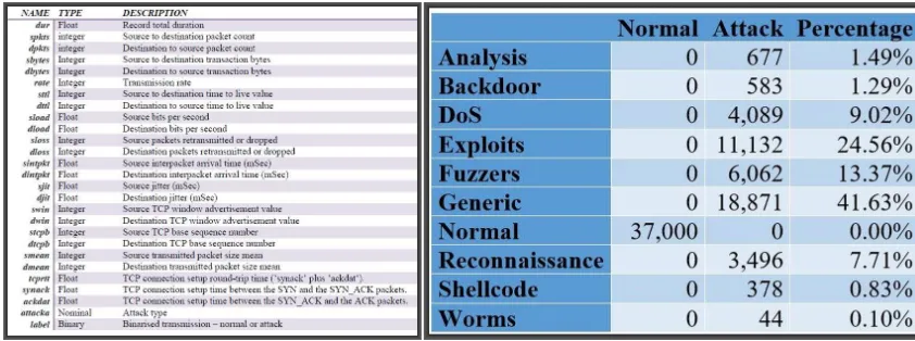
Table 1: Data attributes and class labels (LHS) and summary of the UNSW-NB 15 data flow types (RHS)

The right hand side (RHS) panel exhibits ninemaliciouscategories and onenormal. The former takes two forms–binomial and multinomial–forming a good data source for multiple sampling, training and testing. To fulfil the foregoing ob-jectives, sampled subsetsxi[τ]whereτis an indicator of sample sizes are extracted for natural grouping.

3.2

Modelling Strategy

The samples are used to form natural groupingsCiτ each with a notional probabilityπk[τ]such thatPK_k=1πk[τ],

wherek = 1,2, . . . K is the number of groups and the p−dimensional probability function p(xτ,j, ωk)is fully

described by the distributional parametersωk. Throughout the samples, one parameter of interest is

ξτ=

Pn

i=1zˆi,k[τ]

Pn

i=1zˆi,k[τ] +P n

i=1zˆi,k¯[τ]

∝

K

X

k=1

πk (2)

wherezˆi,k[τ]is an indicator variable denoting membership to groupkor otherwise andτ = 1,2,3. . . mis the sample

number. Now, consider a case from a completely random traffic in whichna = Pn_i=1zˆi,k[τ]is the total number of

cases identified as malicious andn−na =Pn_i=1(1−zˆi,k[τ]).Given random sampling, a natural estimator for the

averagenormalflow effect can be presented as the difference in the average outcomes of the cases identified asnormal

versus identified asmalicious. The parameter of interest in Equation 2 leads to the expression in Equation 3.

1 n n X i=1 _zˆ

i,k[τ]xi,k[τ] na

n

−(1−zˆi,k_n−) [_nτ]xi,k[τ]

a

n

∝ξτ (3)

Since every sample is fixed, randomness only manifests in the componentzˆi,k[τ]and subsequently inξτ ∝πk.Thus,

the main idea of our strategy is that, by treating membership to these group proportions as missing data and repeatedly sampling and validating clusters, we characterise the overall behaviour of cyber-intrusion. That is, givenxτas defined

above, we can separatekgroups with probabilities πk andπ¯k corresponding to different descriptions of intrusion.

Correlation analysis, Principal Component Analysis (PCA) and Kernel Density Estimation (KDE) are well-known conventional methods that can be applied to analyse the variations in Equation 3. In particular, the KDE, defined as

ˆ

fβ(xiτ) =

1

β n

X

i=1

Kβ(ˆziτx−xiτ) =

1

nβK

_zˆ

iτx−xiτ β

(4)

whereRKβ(ˆziτx−xiτ) = 1 is zero-centred and the key parameterβ > 0 determines the number of emerging

structures in the sample and therefore its optimal value is proportional to the variations betweenˆzi,k and1−zˆi,k.

4. RESULTS AND DISCUSSIONS

for. For thenτ×pmatrix from each sample, we can compute matrixV which diagonalises the covariance matrixΣ

such thatV−1ΣV=G,whereGis a matrix of theeigenvaluesofΣ.The columns ofVareorthorgonalto each other and they define the principal components whereas the diagonal values ofGare the variances of the components. The orthogonalVare theeigenvectors, i.e., uncorrelated data with directions and magnitude defining each component.

As far as optimising variation in data is concerned,βandeigenvaluesplay a similar role and so, in both cases, we can optimise their expected values via repeated sampling. For example, through each sample we can generate a correlation matrix that is re-ordered based on the angular order of the eigenvectors as defined in Equation 5.

ρi,τ =

 



tanei,2

ei,1

, if ei,1>0

tanei,2

ei,1

+π, if ei,1<0

(5)

wheree1ande2are the largesteigenvaluesfrom the matrix. The mechanics for implementing the foregoing strategy

in pursuit of the objectives outlined in Section 1 are presented in a finite number of steps in Algorithm 1.

Algorithm 1

1: procedureOPTIMALVARIATION(OPTIVA) 2: Load xi,j⊂Ω.

3: Set: S[τ] =s1, s2, . . . sm (Sample sizes vector of lengthm).

4: Init: Φρ(.) = Ø (Correlation Storage Matrix).

5: Init: L(.) = Ø (Loadings/Directions Storage Matrix).

6: Init: ∆L(.) = Ø (Sample-based Variations in Loadings/Directions).

7: whileµ≤mdo

8: Updateµ:=µ+ 1.

9: Sτ ←zˆi,jxi,j[τ]⊂Ω.

10: UpdateΦτ(.)←ρi,τ ← Sτ.

11: UpdateLτ(.) ←

n

vj,τ; gj,τ; dj,τ

Pn i=1di,τ

o

← Ci,j[τ].

12: Update∆L(.) ← +₋{Lµ− Lµ+1}.

13: forη= 1→dimLi,jdo

14: CA∆,τ =

Pµ ι=1∆L(.)

µ ⇐⇒

∆Lµ+1(.)+µCA∆,µ

µ+1 =CA∆,µ+1 (Cummulative Moving Average).

15: Plot CA∆,µ+1[j, τ] (For Validation).

16: Store CA∆,µ+1[j, τ].

17: Store Lµ(Dom) ← CA∆,µ+1[j, τ] (Dominant Loadings).

18: end for

19: end while

20: Output and interpretCm,i,j[τ].

21: end procedure

The algorithm repeatedly takes up tomsamples of different sizes, spacing and order fromΩ.The magnitudes can be determined via exploratory analyses but the order is not particularly important. The algorithm’s main idea is to compare variations in rotations - the quantities which form the principal components. Averaging of the variations may be confined to a few components contributing to the highest variation in data or may include allj=pcomponents.

4

Results and Discussions

4. RESULTS AND DISCUSSIONS

4.1

Preliminary Analyses

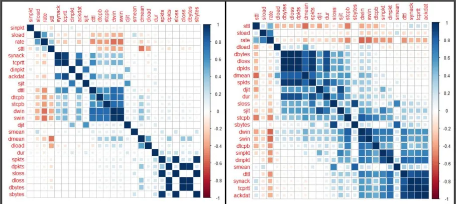
The two panels in Figure 1 exhibit correlation structures among the transmission variables. They both provide insights into how different transmission parameters interact based on which we can adjust the sampling parameters mentioned above. The RHS panel provides an ordered visual pattern that can be useful further analyses as in PCA below. Figure 1

Figure 1: Full data correlogram (LHS) and one for sample size 50 (RHS)

exhibits two extreme cases of the variable correlations based on the number of observations. In both cases it is evident that the variablesdpkts, dlossanddbytesare highly correlated–almost perfectly positive. The same can be said of

synackandtcprtt;tcprttandackdatas well asspkts, sloss, sbytes. While there aren’t many extreme cases of high correlation in the full dataset, samples drawn from it indicate high multicollinearity among the variables. Interpretation of principal components, discussed below, is preceded by computations of correlations between the original data for each variable and each extracted component. It is worth noting that interpretation of the principal components is based on finding the variables which most correlate with the components, as discussed below.

4.2

Extracting, Interpreting and Optimising Principal Components

The panels in Figure 2 represent the same plot of the first two components from the full data labelled by all type of data flows on the left and by the binarised flow on the right. By theeigenvalue rulewe can accept 8 components which have a value greater than 1. The first eight components account for 81.34% of variation in the original data with the first through eighth accounting for 24.3%, 14.4%, 11.55%, 8.97%, 8.48%, 5.15%, 4.28% and 4.19% respectively. We see, on the left hand side panel, that there is a clear separation of attributes that describeExploits,DosandGeneric

4. RESULTS AND DISCUSSIONS

Figure 2: Two panels of the same plot with multi-class and binary labelling

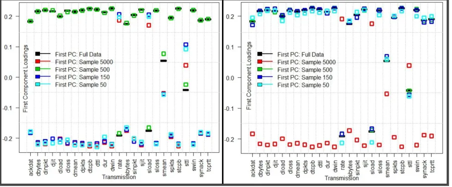
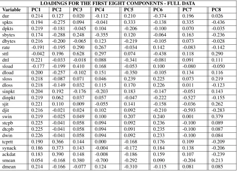
Loadings of the first eight components from the full data are presented in Table 2, where it can be seen that there is no single very high correlation between the variables and the extracted components. The magnitudes and directions of the loadings underline the existing multicollinearity among the data flow variables which can also be explained by the large number of components extracted. These metrics represent the influence of the individual variables in constructing the component and, hence, by repeatedly sampling and extracting new components we generate a range of new metrics which can be aggregared and averaged in line with Algorithm 1.

Figure 3: Selected runs for first component patterns generated by the full data and different sample sizes

4. RESULTS AND DISCUSSIONS

LOADINGS FOR THE FIRST EIGHT COMPONENTS - FULL DATA

Variable PC1 PC2 PC3 PC4 PC5 PC6 PC7 PC8

dur 0.214 0.127 0.020 -0.112 0.210 -0.374 0.196 0.026 spkts 0.194 -0.275 0.094 -0.041 0.333 -0.138 0.335 -0.436 dpkts 0.219 -0.181 -0.045 0.104 -0.206 -0.100 0.070 -0.035 sbytes 0.174 -0.288 0.248 -0.355 0.120 -0.064 0.163 -0.236 dbytes 0.216 -0.200 -0.065 0.123 -0.219 -0.105 0.073 -0.028 rate -0.191 -0.195 0.290 0.267 -0.034 0.142 -0.083 -0.142 sttl -0.042 0.196 0.628 0.297 0.074 -0.438 0.118 0.290 dttl 0.221 -0.033 -0.018 0.088 -0.341 -0.081 0.091 0.111 sload -0.177 -0.199 0.410 0.168 -0.053 0.100 -0.080 -0.050 dload 0.200 -0.257 -0.102 0.151 -0.350 -0.105 0.134 0.116 sloss 0.218 -0.087 0.071 0.046 0.239 0.225 0.073 0.219 dloss 0.218 -0.149 0.032 0.115 0.170 0.226 0.011 -0.123 sinpkt 0.204 0.192 -0.176 -0.203 0.183 -0.147 -0.051 0.143 dinpkt 0.219 0.062 0.037 0.057 -0.047 -0.222 -0.527 -0.155 sjit 0.221 0.110 0.009 -0.055 0.141 -0.158 -0.036 0.262 djit 0.216 -0.021 0.024 0.102 0.092 -0.210 -0.593 -0.283 swin 0.219 -0.025 0.049 0.100 0.207 0.240 0.001 0.379 stcpb 0.225 -0.041 0.058 0.094 0.092 0.236 -0.100 0.089 dtcpb 0.225 -0.041 0.058 0.094 0.091 0.235 -0.100 0.087 dwin 0.226 -0.041 0.058 0.094 0.092 0.233 -0.100 0.084 tcprtt 0.190 0.366 0.144 0.000 -0.168 0.176 0.109 -0.209 synack 0.186 0.373 0.143 -0.004 -0.172 0.184 0.138 -0.206 ackdat 0.183 0.390 0.148 -0.008 -0.186 0.159 0.107 -0.239 smean 0.054 -0.168 0.380 -0.700 -0.292 0.090 -0.204 0.213 dmean 0.214 -0.166 -0.077 0.124 -0.310 -0.115 0.081 0.085

Table 2: Loadings of the first eight components accounting for 81.34% of the variation in the original data

4. RESULTS AND DISCUSSIONS

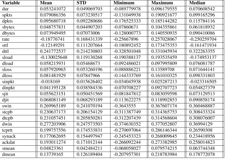
Variable Mean STD Minimum Maximum Median

dur 0.053241072 0.049069703 -0.089779978 0.096179555 0.070608542 spkts 0.079086356 0.073230517 -0.131049938 0.190921677 0.099165296 dpkts 0.095680718 0.092280686 -0.176525333 0.185144282 0.115784116 sbytes 0.048757831 0.044907203 -0.07860671 0.104355861 0.061818932 dbytes 0.073949495 0.07073006 -0.128000773 0.140550935 0.090410086 rate -0.18776741 0.168431339 -0.25667896 0.257028067 -0.250259704 sttl -0.12149291 0.111207664 -0.180892452 0.173475353 -0.161471934 dttl 0.241772537 0.214230803 -0.328501048 0.331045934 0.322263355 sload -0.130025648 0.119130268 -0.190388137 0.193535459 -0.174953137 dload 0.058215931 0.05468673 -0.092486021 0.097995809 0.076081787 sloss 0.057920965 0.053260196 -0.088886221 0.13589708 0.071644141 dloss 0.081481929 0.07847966 -0.144333769 0.161010325 0.098331803 sinpkt -0.018169 0.015626402 -0.034045938 0.025287213 -0.023316505 dinpkt 0.041195128 0.038584336 -0.070708227 0.092707723 0.054827379 sjit 0.055623151 0.050451569 -0.081847812 0.083059598 0.073129513 djit 0.068081149 0.068293189 -0.113622275 0.118902853 0.090858174 swin 0.269965189 0.241070194 -0.3643555 0.367607174 0.360468887 stcpb 0.230637173 0.206154129 -0.311387749 0.314365753 0.308433324 dtcpb 0.231057451 0.205850281 -0.312207439 0.314568604 0.308076007 dwin 0.277203906 0.247573503 -0.374630352 0.377052807 0.36994129 tcprtt 0.199757556 0.174533831 -0.270697064 0.286146344 0.26590308 synack 0.177062695 0.154497947 -0.245453323 0.268009645 0.234418956 ackdat 0.193011274 0.171012144 -0.266092244 0.273382985 0.258014823 smean 0.04823361 0.042484211 -0.068058027 0.079574215 0.063744348 dmean 0.13739165 0.126189404 -0.207957301 0.218783984 0.178772078

Table 3: Descriptive statistics of each of the 25 component forming variables across 40 samples

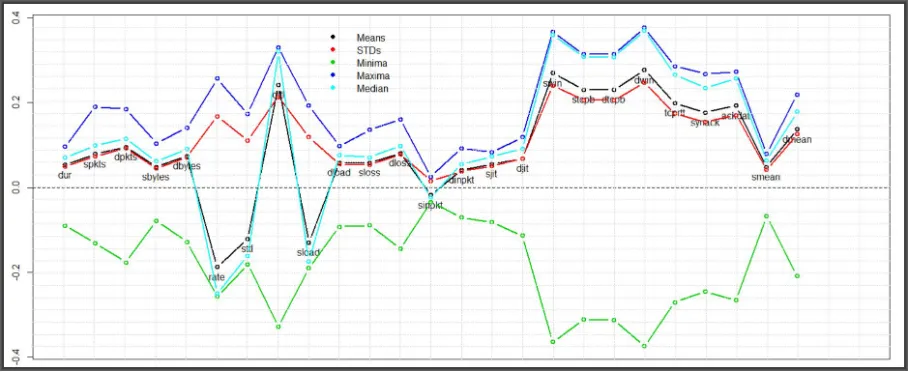
The parameters used in constructing Table 3 and Figure 4 are proportional to the coefficients of the linear combination of the original variables in Table 1. The linear combination makes up PC1 and, in this particular application, they impinge on the nature of the traffic and so they can be used as predictors of the phenomenon that they symbolise. The degree of influence of each variable in constructing the components can be deduced from both Tables 2 and 3 as well as from Figure 4. As implied by Equation 3, randomness manifests in sampling and, hence, in the calculation of

5. CONCLUDING REMARKS

Figure 4: A graphical illustrations of the malicious flows descriptive statistics in Table 3 from across 40 samples

Both the original full data and repeated samples exhibit a clear pattern of duality. The left hand side panel in Figure 5 shows the densities of the full data and three random samples of sizes 50, 500 and 5000 while the patterns on the right are proportional to the correlations between the individual variables and the first component across 40 samples.

Figure 5: Component one densities from selected samples and 40 samples variable correlations with the component

The fact that no single variable exhibits significantly high correlation with the component in the right hand side panel of Figure 5 highlights the potential masking of the flows. However, the fact that together the variables show a consistent separation of the data into two distinctive regions, with several variables such as dttl, sttl, dload, rate, dlossetc, standing out, implies that based on patterns and relationships from both the full data and multiple samples drawn from it–i.e., givenxτ as defined in Section 3.1, we can separatekgroups with probabilitiesπk andπ¯_k corresponding to

different descriptions of intrusion. More specifically, we can use historical data numerics associated with the first significant components, say, to train and test models to measuring and monitoring the risk of known types of intrusion.

5

Concluding Remarks

5. CONCLUDING REMARKS

the two well-documented intrusion detection techniques -misusein [17] andanomalydetection [18]. Our modelling interpretation of the former is that of rule-based decision that would help identify a suspicious behavior by comparing it to known catalogued malicious flows. On the other hand, the latter, as in many applications, was perceived as a model, the departure from which is a cause for alarm. We took a unified approach to the two and in both cases the binary and multi-class labels in the dataset used in the study provided the basis for such an approach. Comparing the performance of our method of choice, PCA, with other dimensional reduction techniques would have been ideal, but for the limitations imposed by the study objectives. However, we were able to demonstrate, via Algorithm 1, how information resulting from reduced data dimension of a large number ofmaliciousflows, can be utilised to monitor the emerging structures and potentially be used as inputs in build robust intrusion detection systems. The results were achieved via repeated sampling, yielding parameters that were generally used to fine-tune potential structures in each sample. Aggregating the parameters over many runs, we were able to reproduce consistent patterns of the data dual-ity. The resulting patterns render themselves readily to predictive modelling using the two class labels and therefore provide scope for extension into identifying new attacks. For that to happen, however, data attributes must always be added to the training and testing set repositories, not least because of the dynamic nature of intrusion.

Novelty of our approach derives from iterative estimation of the roles played by individual variables in construction of components, particularly the potential for monitoring future attacks by focusing on the metrics that dominate the components. Without being influenced by the provided levels of attack types, our findings are particularly intriguing for two reasons–the duality may mean either masking or swamping of attack types. That is, some currently unknown attack types may slip through as normal which is why it is imperative to highlight two important aspects of this study–the mechanics of the algorithm and the data attributes. If we knew the relevant density functions and classes of attack, we would simply observe data flows and make predictions. But in practice we have to estimate these parameters from random data and test our algorithms on another random dataset. Our contribution focused on variability as determined byzi[τ]and proportionsπk. For continuous attributes, these parameters typically derive from the mean

REFERENCES

References

[1] S. Wu and W. Banzhaf. The use of computational intelligence in intrusion detection systems: A review. Applied Soft Computing, 10(1):1–35, 2001.

[2] R. Sommer and V. Paxson. Outside the closed world: On using machine learning for network intrusion detection.

IEEE Symposium on Security and Privacy, 2010.

[3] S. Suthaharan. Big data classification: Problems and challenges in network intrusion prediction with machine learning.SIGMETRICS Perform. Eval. Rev., 41(4):70–73, April 2014.

[4] Y. Demchenko, C. Ngo, C. de Laat, P. Membrey, and D. Gordijenko. Big security for big data: Addressing secu-rity challenges for the big data infrastructure. InSecure Data Management, pages 76 – 94. Springer International Publishing, 2014.

[5] L. Kaufman. Can public-cloud security meet its unique challenges? IEEE Security & Privacy, 8:55–57, 2010.

[6] W. Lee, S. Stolfo, and K. Mok. Adaptive intrusion detection: A data mining approach. Artificial Intelligence Review, 14:533 – 567, 2000.

[7] S. Noel, D. Wijesekera, and C. Youman. Modern intrusion detection, data mining, and degrees of attack guilt.

Applications of Data Mining in Computer Security: Advances in Information Security, 6:1–31, 2002.

[8] R. Mitchell and I-R. Chen. Behavior rule specification-based intrusion detection for safety critical medical cyber physical systems.IEEE Transactions on Dependable and Secure Computing, 12:16–30, 2015.

[9] M. Maechler, P. Rousseeuw, A. Struyf, M. Hubert, and K. Hornik. cluster: Cluster Analysis Basics and Exten-sions, 2013. R package version 3.4.0.

[10] K. V. Mardia, J. T. Kent Kent, and J. M. Bibby.Multivariate Analysis. Academic Press, 1979.

[11] N. Kambhatla and T. Leen. Dimension reduction by local principal component analysis. Neural Computation, 9:1493–1516, 1997.

[12] K. Mwitondi, C. Taylor, and J. Kent. Using boosting in classification.Proceedings of the Leeds Annual Statistical Research (LASR) Conference; Leeds University Press, pages 125–128, 2002.

[13] K. Mwitondi, R. Moustafa, and A. Hadi. A data-driven method for selecting optimal models based on graphical visualisation of differences in sequentially fitted roc model parameters. Data Science, 12:WDS247–WDS253, 2013.

[14] K. Mwitondi and R. Said. A data-based method for harmonising heterogeneous data modelling techniques across data mining applications.Statistics Applications and Probability, Pro 2(3):293–305, 2013.

[15] N. Moustafa and J. Slay. Unsw-nb15: A comprehensive data set for network intrusion detection systems.Cyber Range Lab of the Australian Centre for Cyber Security (ACCS), 2015.

[16] N. Moustafa and J. Slay. The evaluation of network anomaly detection systems: Statistical analysis of the unsw-nb15 data set and the comparison with the kdd99 data set. Security Journal: A Global Perspective, pages 1–14, 2016.

[17] S. Kumar and E. Spafford. A software architecture to support misuse intrusion detection. Proceedings of the 18th National Information Security Conference, pages 194–204, 1995.