Lattice Boltzmann simulation methods for boundaries and interfaces in multi component flow

(1)

Lattice Boltzmann simulation methods for boundaries and

interfaces in multi component flow.

HOLLIS, Adam P.

Available from Sheffield Hallam University Research Archive (SHURA) at:

http://shura.shu.ac.uk/19815/

This document is the author deposited version. You are advised to consult the

publisher's version if you wish to cite from it.

Published version

HOLLIS, Adam P. (2009). Lattice Boltzmann simulation methods for boundaries and

interfaces in multi component flow. Doctoral, Sheffield Hallam University (United

Kingdom)..

Copyright and re-use policy

(2)

I Adsetts Centre City Campus

L

Sheffield S1 1WB

1 0 1 9 0 7 5 7 2 4

III I I llllll

r o h e ^ e id Haitem University

i Leaminq and IT Services

Aosetts Centre City Campus

(3)

ProQuest Number: 10697121

INFORMATION TO ALL USERS

The quality of this reproduction is dependent upon the quality of the copy submitted.

In the unlikely event that the author did not send a com plete manuscript and there are missing pages, these will be noted. Also, if material had to be removed,

a note will indicate the deletion.

uest

ProQuest 10697121

Published by ProQuest LLC(2017). Copyright of the Dissertation is held by the Author.

This work is protected against unauthorized copying under Title 17, United States C ode Microform Edition © ProQuest LLC.

ProQuest LLC.

789 East Eisenhower Parkway P.O. Box 1346

(4)

Lattice Boltzmann Simulation Methods for

Boundaries and Interfaces in Multi Component

Flow.

Adam Peter Hollis.

A thesis submitted in partial fulfilment of the requirements of

Sheffield Hallam University for the degree of Doctor of Philosophy

Materials Research Institute, Sheffield Hallam University, Howard

Street, SI 1WB, UK

(5)

Abstract

(6)

Acknowledgments

I would like to express my gratitude to my supervisory team Dr. Ian Halliday who inspired me throughout this work and my undergraduate studies and Prof. Chris Care for their assistance and guidance through the course of this work.

Fluent Europe Ltd to whom I am very grateful has provided funding for my research.

I would like to thank my external examiner Dr Rammille Ettelaie and my internal examiner Prof Marcos Rodrigues who very kindly agreed to be my examiner at short notice.

I would finally like to thank my family but especially my parents Margaret and Peter Hollis for their continued support, both financially and emotionally, and instilling me with the .confidence and drive to complete this work.

(7)

Publications

Below is a list of publications to date:

• I. Halliday, R. Law, C.M. Care and A. Hollis. Improved simulation Of drop dynamics in a shear flow at low Reynolds and capillary number. Phys. Rev. E, 73, 056708, (2006).

• A. Hollis, I. Halliday and C.M. Care. Enhanced, mass^conserving closure scheme for lattice Boltzmann equation hydrodynamics. J. Phys. A: Math. Gen. 39, 10589 - 10601, (2006).

• I. Halliday, A. Hollis and C.M. Care. Lattice Boltzmann algorithm for contin uum multi-component flow. Phys. Rev. E, 76, 026708, (2007).

• I. Halliday, A. Hollis and R. Law . Kinematic condition for multi-component lattice Boltzmann simulation. Phys. Rev. E, 76, 026709, (2007).

• A. Hollis, I. Halliday and C.M. Care. An accurate and versatile lattice closure scheme for lattice Boltzmann equation fluids under external forces. J.Comp. Phys. 277, 17, (2008)

• Lawford P.V, Ventikos Y, Khir A.M, Atherton M., Evans D, Hose D.R, Care C.M, Watton, P.N, Halliday I, Walker D.C, Hollis A.P, Collins M. Modelling the Interaction of Haemodynamics and the Artery Wall: Current Status and

(8)

5 Mass Conserving Boundary Closure Scheme

59

5.1 Introduction... . 59

5.2 Aspects of Lattice Boltzmann Theory ... . 61

5.3 Mass Conserving Lattice Closure A lg o rith m ... 61

5.3.1 Planar Boundary A lg o rith m ... 62

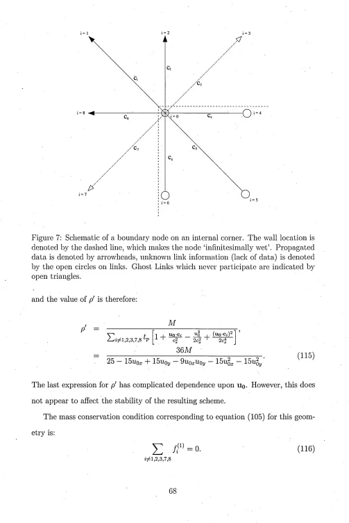
5.3.2 Internal Corner Algorithm . ...67

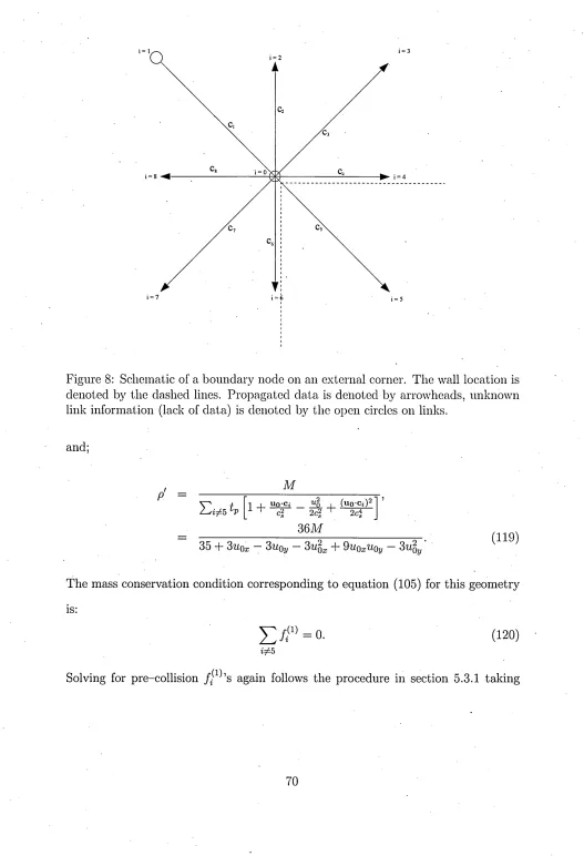
5.3.3 External Corner Algorithm ... 69

5.4 Initial Comments on Boundary F o rcin g... . 72

5.5 Results ... 72

5.6 C om m ents... . 78

6 Mass Conserving Boundary Closure Scheme for Fluids Subject to

External Forces

79

6.1 Introduction ... 79

6.2 Further Background to LB Dynamics . . . ... 81

6.3 Limiting Assumptions ...84

6.4 Lattice Closure Algorithm for Fluid at a Boundary Subject to a Con stant External Force 84

6.4.1 Planar Boundary A lg orith m ...85

6.4.2 Internal Corner A lg o rith m ... 93

(10)

6.5 R esults . . ; ... 96

6.6 S u m m a ry ... 104

7 Simulation at Low Reynolds and Capillary numbers for M

ulti-Component LB

107

7.1 Preliminary R em ark s... 107

7.2 Background and Context ... 108

7.3 Problems Associated with Reduced Reynolds and Capillary Number Simulations Using MCLB ... 110

7.4 Multi-component Lattice Boltzmann in the Continuum Approximation 114 7.5 Improvements to the M o d e l... ... 116

7.5.1 Interface Source T e r m ... ... . . . . . 116

7.5.2 Interface Definition and Cumulative Forcing . . . 118

7.5.3 Calculation of Numerical D erivatives...121

7.6 Kinematic condition ... . 123

7.6.1 Kinematic P ro b lem ... 123

7.6.2 Kinematic Condition Solutions ... 124

7.6.3 Com m ents... 125

7.7 R esults... 126

7.7.1 Simulations of drop lift in shear f l o w ...126

7.7.2 Kinematic c o n d itio n ... 130

7.8 D iscussion... 132

7.9 Conclusion . . . ... 136

7.10 Chapter Summary ... 137

8 New Approach to Continuum MCLB Simulation

139

• 8.1 Preliminary R em ark s... 139

8.2 Introduction... 140

8.3 Interfacial Hydrodynamics in the Continuum ap p ro x im atio n ...141

(11)

8.4 Multi-component lattice Boltzmann in the continuum approximation 142

8.5 Analysis of the Formulaic Segregation R u le ...146

8.6 Acceleration of Colour Flux . ... 149

8.6.1 Planar Interface at R e s t ... 152

8.6.2 Curved In te rfa c e ... 154

8.7 Stability of the Interface ... 156

8.8 Dynamics of the Phase Field ... 159

8.9 Local Expression For Colour G radient... . . ... 169

8.10 Results ... 172

8.11 Conclusion...175

9 Kinematic Condition for Distributed Interface

177

9.1 Introduction ... 177

9.2 B ackground... 178

9.3 Kinematic C o n d itio n ... 180

9.4 Results and conclusion ... 183

10 Wetting with continuum IB :

Simulation of 2D dense Films Under

Gravity

187

10.1 Introduction... ... ... • 187

10.2 Background . . . ... 188

10.3 General Remarks on the Implementation of the Slip Condition . . . . 192

10.4 Application of Formulaic Segregation at a Forced Boundary Node with S lip ... • 193

10.4.1 Effective Red and Blue Fluid Densities for Boundary Node . . 194

10.5- Stress Measurements with Spatially Variable Force ... 196

10.6 R esults... 197

(12)

11 Prospective Future Work

205

11.1 Introduction... 205

11.2 Curvature D isco n tin u ity... 205

11.3 Possible Solution ... 207

(13)

1 Thesis Overview

Work carried out as part of this report has been supported by Fluent Europe Ltd. Although some of the nomenclature and language used in this section are yet to be explained; it is deemed appropriate at the outset to provide an overview of the aims and objectives of the work and to outline the intended route to fulfilling these. This section shall detail the initial issues associated with the inherited multi-component lattice Boltzmann method and the steps taken to overcome these issues. The layout of the thesis shall also be described.

1.1 A im s of thesis

At the beginning of this work the multi-component lattice Boltzmann (MCLB) method showed great potential in a number of important areas of continuum flow calculations. However there remained a variety of significant problems within the core method, see Chapter 7 for an in-depth analysis of the associated problems with the core method.

The major issues that are to be addressed within this work may be summarized as follows:

1. Micro-currents on multi-component interface obscuring hydrodynamic signals.

2. Lattice pinning in low Reynolds number flows or “sticking to the simulation

lattice” of the multi-component interface.

3. Indeterminate interfacial hydrodynamics and a verifiable absence of a kine matic condition.

4. Verifiable contact line behaviour at an accurately represented boundary with the ability to recover Navier conditions.

(14)

The intended aim of this project was to improve and develop lattice Boltzmann simulation of multi-component immiscible fluids, with particular attention being paid to the above issues, thus facilitating simulations in micro-fluidic regimes and venule scale blood flow applications. It is stressed at the outset that individual application of the method to a specific situation is not the purpose of this work. The ultimate aim is to produce an effective and accurate LB method for the simulation of interface-dominated flow including wetting in both static and dynamic conditions.

1.2 Layout

Considering the issues arising in the inherited model that were identified in the previous section; it is clear that the work devolves into two sections.

1. Consideration of boundary conditions.

2. Fundamental issues arising from MCLB interfaces.

In terms of the structure of the thesis I intend to address the above issues as follows: I initially intend to address the issue of boundary conditions exhaustively. For tractability and for my own personal introduction into the subject it was decided that boundary conditions are, initially, to be examined using single component lattice Boltzmann (SCLB).

Having resolved any issues arising while working on- an accurate and effective boundary condition; the remaining problems that are associated with the MCLB interface shall be resolved.

Finally the two work-packets listed above shall be combined in order to create an effective algorithm for the treatment of multi-component fluids at solid boundaries. Having done this the issues raised in items 1-4 in 1.1 above will have been resolved.

Considering the above discussion the structure of this thesis is as follows: Following an introduction in Chapter 2; Chapters 3 and 4 highlight all relevant background material used in subsequent chapters. Relevant fluid mechanics is briefly

(15)

discussed in Chapter 3 with relevant lattice methods reviewed in chapter 4. It is noted here that this is not intended to be a complete treatment of fluid mechanics but a brief overview intended to put the work into context.

Chapters 5 and 6 contain a rigorous treatment of the issues arising with boundary

conditions. This treatment of boundary closure methods is carried out using SCLB initially. It will be generalized later in Chapter 10.

Chapter 7 details my initial attempts using an inherited MCLB. The issues highlighted in points 1-3 in 1.1 are addressed with only partial success. This chapter serves to highlight the inadequacies of the core model that I inherited.

Chapters 8 and 9 contain a fundamental revision to the core MCLB algorithm

which proved successful in overcoming the issues of 1-3 in 1.1.

Chapter 10 attempts to combine advances made in SCLB from chapters 5 and

6 with the MCLB advances made in chapters 8 and 9. The aim of this chapter is

to show how a flexible method has been developed for boundary closure, that is capable of dealing effectively with interfaces and Navier slip conditions.

Chapter 11 proposes future work and extensions to the new methods and suggests

(16)

2 Introduction

Fluid dynamics is a branch of physics and mechanics dealing with fluids, these can be liquid i.e. hydrodynamics or gaseous i.e. aerodynamics. The effects of fluid motion impacts upon us within most areas of our daily lives from aerodynamics within automotive industries to pharmaceutical manufacture ensuring even distri bution of components drug mixing within crucibles. A conventional approach within engineering environments is to recreate flow phenomena through the use of certain dimensionless numbers, that are discussed later. Using these dimensionless parame-' ters it is possible to physically recreate various flow environments through ‘dynamic similitude’. In other words, real systems may be classified by dimensionless numbers so as to recreate identical fluid effects using different physical models described by the same numbers. Such concepts are used in practical experiments such as wind tunnels etc. Physical scaling of systems is an effective way of reproducing fluid phenomena within flow domains however there are also various disadvantages to dynamic similitude. Conducting physical dynamic similitude experiments is a time consuming and costly process, making minor changes to the flow domain can be difficult, quantitative data may only be collected from discrete points within the simulation domain giving local information only. Additional complications arise when conducting dynamic similitude experiments when various flow regimes are to be analysed for example laminar or turbulent flow, difficulties can arise in produc ing identical experimental conditions for both flow regimes. Computational fluid dynamics packages therefore offer a cost effective, transportable and adaptable way of simulating systems to aid understanding of physical experiment or to simulate sys tems that may be too complex for dynamic similitude experiments. In conjunction with theoretical fluid mechanics, the three methods allow us to better understand the processes taking place within flow systems.

In respect of the computation methods at the heart of this thesis, the first

(17)

tempt to model fluid flow successfully and recover the rotational symmetry of the Navier-Stokes equations was made in 1986 by Uriel Frisch, Brosl Hasslacher and Yves Pomeau (FHP) [1] when they produced a cellular automaton (CA) computer simulation that worked by obeying conservation laws to recover hydrodynamics on a microscopic level. This early CA worked using a two step mechanism, a free-stream and a collision; the free-stream operation involves the movement of Boolean parti cles from one site on a hexagonal lattice to an adjacent lattice site, thus making the method a Lattice Gas Cellular Automation (LGCA). The collision step occurs when Boolean particles reach the same site on the lattice at the same time and interact; the total momentum is conserved but redistributed between the particles at that site. The redistribution is governed by a set of local collision protocols. This system is clearly, time-space discretised.

Due to the large amounts of integers being processed for a Boolean LGC A sim ulation there is inevitably large amounts of statistical noise. In an effort to try and reduce the levels of statistical noise and recover behaviour more conclusively related to Navier-Stokes behaviour, the Boolean components were replaced with, effectively, an ensemble-average population based on a distributed Maxwell-Boltzmann distri bution! It was soon realized that the technique of replacing the Boolean particles and integer arithmetic with floating point arithmetic on continuous populations was a valid method of reproducing fluid hydrodynamics in its own right [2]. Hence the first form of the Lattice Boltzmann Equation (LBE) was produced.

Fluid mechanics relies on the laws of conservation, in this report the Lattice Bhatnagar Gross and Krook (LBGK) algorithm will be used for the implementation of the Boltzmann equation on a lattice. The algorithm is implemented on a two dimensional lattice with nine possible velocities (D2Q9) that will be covered in more detail later. [3] [4]

(18)

viscosity. The fluids are viewed in the continuum regime or in other words are considered to be continuously divisible. The interaction of the individual particles comprising the fluid are not directly considered. Thus physical parameters such as the velocity of the fluid and the fluid density may be specified at any point within the flow domain.

Throughout this work, flow shall be regarded as incompressible and isothermal. All fluids are compressible to some degree however the assumption of incompressibil ity allows us to assume a constant density throughout the continuum fluid and thus a uniform viscosity. As the fluids are considered to be isothermal we assume them to have a uniform temperature throughout. Consideration of isothermal and incom pressible fluids allows us to greatly simplify the equations governing flow. There has been substantial work carried out considering the energy equation that governs flow [5], as we are considering isothermal and incompressible fluids, this shall not be considered.

The law of mass conservation will be used to derive the Continuity equation and the conservation of momentum will be shown to give rise to a set of three equations known as the Navier-Stokes equations. The Continuity and Navier-stokes equations can be used to describe the behaviour of any fluid within a flow domain, the unique characteristics of the flow are a consequence of the interaction of the fluid with domain boundaries and interface interactions between immiscible components.

Accurate representation of the domain boundaries including the interface be tween two immiscible fluids is therefore essential if accurate hydrodynamics are to be recovered.

2.1 R ecent R elated Advances U sing Lattice B oltzm ann

Throughout this work various recent developments in LBE modelling are directly utilised and are referenced where appropriate such as M.Latva-Kokko and D.H.

(19)

Rothman’s segregation method [6] which was published in 2005. In order to illustrate and contextualize recent developments and to show wider applications of the method I would like to give a brief overview of recent work carried out by G. Berk Usta and Alexander Alexeev from the Chemical Engineering Department of the University of Pittsburgh [7]. The following application illustrates the broader context of the detailed work undertaken in this thesis.

Usta’s work builds on earlier simulation techniques of Alexander Alexeev et al [8].

Alexeev uses two different meso-scale models and integrates them in order to simu late the behaviour of micro-capsules in a continuum fluid. The aim of Alexeev’s work is to combine an LB method fairly similar to ours and a lattice spring method [9] (which will not be discussed in this work), .to simulate the behaviour of a continuum fluid alongside a micro-capsule’s elastic shell. The work aims to improve the speed at which chemical data can be retrieved from micro-reactors. The aim is to ma nipulate minute quantities of reagents that are contained within the micro-capsules. Alexeev also notes that the fluid-filled elastic shelled micro-capsules can also be used as simple models for biological cells such as leukocytes.

Using similar boundary conditions to those developed by Alexeev et al [8] de scribed above; Usta has recently published work describing how, by using the com bined LB and lattice spring method of Alexeev, they have been able to simulate the self propelled motion of micro-capsules.

Usta describes how in some biological systems there is communication between cells which are designated signalling and target cells, this allows the cells to cooperate and thus carry out a large range of functions. The aim of Usta’s work is to mimic the communication that occurs between biological cells. The main outcome is that when considering a pair of cells, one signalling and one target, that are situated in close proximity on a substrate, the action of the signalling cell results in the self-propelled motion of both cells.

(20)

continuum fluid. The signalling cell is filled with dispersed nano-particles within its fluid filled core. These nano-particles are able to diffuse through the shell of the micro-capsule. The nano-particles can “chemisorb” onto the surface of the substrate and modify its wetting properties, in particular its adhesive interaction. The strength of adhesion of the substrate diminishes as the concentration of nano particles chemisorbed onto it increases. The signalling cell therefore emits nano particles that diffuse through the surrounding fluid according to Brownian motion. The deposition of nano-particles on the substrate creates an adhesion gradient em anating from the point directly underneath the centre of mass of the signalling cell. At this stage Usta notes that there is no self-propelled motion as the system is symmetrical.

Placing a target cell in close proximity to the signalling cell however breaks the system’s symmetry. Upon diffusion of the nano-particles, the wetting section of the target cell is exposed to a adhesion gradient. Should the parameter set be appropriate in terms of diffusion rates and relative separation and reactivity of the nano-particles relative to the adhesivness of the surface; the target cell will, under the correct circumstances, move from the less.adhesive area to the more adhesive area, i.e. along the adhesion gradient.

Subsequent to the initial movement of the target cell, Usta found that the hydro dynamics of the continuum fluid caused by the motion of the target cell, initiated movement of the signalling cell itself thus following the target cell along the adhesion gradient. Following this initial movement, both the target cell and the signalling cell lie in asymmetric positions relative to the adhesion gradient and thus continue to move provided that the signalling cell continues to diffuse nano-particles.

Therefore, by utilising the lattice Boltzmann method, Usta et al have designed

a biometric system where communication is achieved between a pair of synthetic particles through the diffusion of nano-particles. They have also shown how the hydrodynamics induced by the target cell can influence the motion of the signalling

(21)

cell thus demonstrating that hydrodynamic forces have an important role in the sensing and signalling behaviour of biological systems.

I will not attem pt simulation with the degree of complexity of Usta et aVs [7] work; my objective is to examine the fundamental accuracy and verifiability of the underlying LB model. However, Usta’s work does illustrate the complexity of the fluid systems that LB can address. The following is the sort of thing that the models I have developed might, eventually, be applied to.

There is a long history of modelling attaching cells as wetting immiscible drops. In the context of this thesis, a similar result to that obtained by Usta et al may be achieved by using the culmination of advances described in this thesis, shown in chapter 10. If simulations of this kind were to be carried out, the wetting properties of the substrate, specifically in the above example, the adhesion properties of the substrate would need to be investigated. In addition, the secondary migration of' the signalling cell that is induced by the hydrodynamics of the continuum fluid must not be compromised by the micro-currents of the interface. The low micro-current interface algorithm demonstrated in Chapter 10 is necessary.

The essential difference between the work in this thesis and that of Usta et

al is our focus on hydrodynamic boundary conditions and their accurate correct

(22)

3 Introduction to Fluid M echanics

The intention here is not to cover fluid dynamics in a comprehensive manner however it is appropriate to consider some key concepts in context; more complete accounts

are to be found in Batchelor [10], Tritton [11], Landau and Lifshitz [5] and Happel

and Brenner [12].

3.1 D im ensionless Q uantities in H ydrodynam ics

In fluid mechanics it is conventional to describe various flow regimes using a variety of different dimensionless quantities. It is appropriate at this stage to mention some of these dimensionless quantities and their meanings. There are a wide range of dimensionless numbers that are applicable to a large variety of flow situations such as; the Nusselt Number (that measures the enhancement of heat transfer within a fluid when convection is considered as well as conduction) and the Schmidt Num ber (that is used to describe the ratio of diffusion of momentum to that of mass). Dimensionless quantities that are to be used regularly in this work are explained below in greater detail.

Throughout this work the following standard notation shall be employed. The shear and kinematic viscosity are denoted as 77 and z/ respectively. The drops we

consider have radius R and surface tension a. Their flow environment is usually

characterised by a velocity Uq and/or a shear rate 7.

3.1.1 Capillary Number

In fluid mechanics the capillary number (Ca) is used when considering the interface between two immiscible fluids or liquid-gas interfaces. The Ca measures the ratio between the effects of viscous forces relative to the surface tension acting across the interface. The Ca may be regarded as the ratio of momentum diffusion forces to

(23)

surface tension forces. The Ca may be expressed quantitatively as follows:

Ca = ^ . (1)

a

Where all symbols have meanings as described previously.

3.1.2 Mach Number

The Mach number (Ma) of a flow may be regarded as a measure of the speed of the flow. It is defined as. the ratio of the speed of an object relative to the fluid and the speed of sound with in the fluid medium. The Ma may be expressed as follows:

M a = — . (2)

Where cs is the speed of sound within the medium and all other symbols have their

usual meaning as described previously.

It is worth noting that the Mach number is temperature dependant as the speed of sound within a given medium varies with temperature. When considered in the context of this work however the Ma may be considered constant as we are solely concerned with isothermal flows.

The Ma is important when considering fluid mechanics simulations as solids being passed by a fluid , at the same Ma will experience similar forces and effects even though the velocity of the passing fluid may not be identical in both cases.

3.1.3 Reynolds Number

(24)

forces in flow to the viscous forces. It may be expressed as the bulk Reynolds number using the dimension of the flow domain or may be expressed as the ‘drop Reynolds

number, the Reynolds number may be used in conjunction with other dimensionless numbers to calibrate simulations of actual systems where dynamic similitude relates different experiments.

3.2 Governing Equations of H ydrodynam ics

3.2.1 Continuity Equation

The Continuity Equation arises as a consequence of the principle of conservation of mass within a flow domain. To illustrate this we can consider a control surface

element of surface area, dA, and its normal unit vector h. If we consider the amount

' of fluid passing through the surface area in a unit time with a velocity u.we have:

Multiplying the above expression through with the density of the fluid gives us an

Now using surface integration techniques and applying the law of mass conservation, the total change in mass of the volume, uq, with surface area, A, must equal the

number’ (Red) which uses the local dimension of a drop contained within flow as

follows;

(3)

(4)

where W is the physical dimension of the flow domain, 7 is the shear rate, R is the

radius of the drop and u is the dynamic viscosity of the fluid. As with the Mach

u.hdA = u.dA\ dA = hdA.

(5)

expression for the mass of fluid passing through the surface element in a unit time.

(25)

amount of mass passing through the surface, 5, in a unit time:

d_

dt p.du = —

i f .

pu.dA. (6)

Using the divergence theorem on the reference volume provided that mass is neither created nor destroyed, we have;

-V(pu)du.

(7)

Equating integrals we obtain from the principle of mass conservation and the diver gence theorem [13];

(

8

)

We have therefore shown that the continuity equation comes as a direct result of the conservation of mass within a system. The continuity equations is the most fundamental equation within fluid mechanics.

3.2.2 Euler Equation .

The Navier-Stokes equations arise from the conservation of momentum and the application of Newton’s second law of motion. The equations are parabolic second- order partial differential equations that are fundamental in fluid mechanics and, along with the continuity equation and the flow boundary conditions, close the description of hydrodynamic flow processes.

Prior to derivation Of the Navier Stokes equations it is appropriate to derive the Euler equation. Which applies to the ideal and reversible flow processes.

Force exerted by a liquid on a material enclosed in a surface “s” is :

(26)

Now, by applying the divergence theorem to the vector V = Va with a a constant unit vector, it is straightforward to show that:

that is;

V.dA = a. VdA = a. V ttfV , (10)

S J Js J J J V

VdA = / / / V Vcrr, (11)

5 J J Jv

which when applied-to equation (9) gives;

F = - [ I P.dA = -

[ f [

(V P)d3r. (12) J J S J J Jv Q

Making the definition for the force per unit volume on the immersed reference body to be:

E =

[ f [

Fldb, (13)

J J J v 0

which may be inserted into equation (12) in order to give the equivalence;

F' = — VP. (14)

Consider Newton’s second law of motion and express it as a material derivative the momentum of the unit volume. Expanding the material derivative we may express the force per unit volume in terms of time and space derivatives:

w D d d d . .

F = P- u = p ( ^ + ux- u + uy- u + uz- u ) . (15)

Compressing the spatial derivatives and making use of the equivalence identified in (14) we can write the Euler equation:

- V P = p{ J + (u.V).u). (16)

(27)

We have derived the Euler equation for an incompressible fluid but it remains true for a compressible fluid also.

3.2.3 Navier-Stokes Equation

We may now proceed to derive the Navier-Stokes equations. Initially we can denote the Euler equation (16) in cartesian tensor form and rearrange with the view of obtaining a form into which we can insert the momentum flux tensor, 11^ [5], and defined below. Taking the Euler equation in tensor notation and rearranging we obtain;

d(ui) dui l d P , ,

= - (u* ^ ) - -p te t- (17)

If we now consider separately the time differential and expand the derivative

using the chain rule we obtain a two term differential equation, if we proceed to replace the density differential on time with the identity proposed by the Continuity equation we can obtain an expression;

duj _ 1 d(puj) Uj d(puk) . .

dt p dt p dxk

Substituting (18) into (17) and rearranging we. obtain,

1 d(puj) Uj d(puk) = duj 1 dP . . .

p dt p dxk Uk dxk pdxi

Rearranging (19) allows us to condense derivatives in xk using the reverse of the product rule for differentiation giving;

dpUj = dP _ dpukUj ■

dt dxi dxk

(28)

equation that will allow us to identify a momentum flux tensor function:

(21)

defining;

f-hfc — P$ik 4" pUfcUii (22) we have;

dpUi _{r 1}_{_} d _TT

r i . r \

ut 'UXk (23)

The momentum flux tensor 11** is defined as the ith component of the momentum

transferred into a reference volume Uq through a surface, S with its normal in the

equation is applicable to ideal fluids only as it represents a momentum transfer mechanism that is totally reversible.

In order to obtain the appropriate hydrodynamics for a non-ideal, viscous fluid, internal friction must be incorporated into the Euler equation (where friction is regarded as dissipation of kinematic energy) which has been expressed in equation (23) in terms of the momentum flux tensor. In order to take account of friction effects the momentum flux tensor is modified, incorporating an additional term,

the viscous stress tensor a'ik. This term introduces momentum dissipation into the

momentum transfer mechanism of the fluid. The modified momentum flux tensor may be expressed as;

Xk direction in a single unit time. It can be noted that the current form of the Euler

(24)

Inserting the modified form of the momentum flux tensor into (22) and substituting

in for n ifc in (23) it is possible to factorize the resulting equation into the following form;

(25)

(29)

The t e r m + a'ik, in (25) is the full stress tensor, and —PSik is known as the hydrodynamic stress component and, as we have discussed, a'ik, is the viscous stress tensor.

From physical arguments the viscous stress tensor must become zero for a fluid that is under uniform translational or rotational motion. From such physical ar guments it is possible to derive an expression for the viscous stress tensor. Such a derivation is carried out in [5] with the result being;

,

dui duk 2 dui

,

£,dui ,oa\

ff* = T,(d ^ + a ^ - 3 dxi + ? (26)

Where 77 and f are coefficients of viscosity and are both positive and functions of pressure and temperature. As we are only considering isothermal and incompressible

flows, these coefficients are constants, tj is known as the shear viscosity and £ is the

bulk viscosity. Substituting into equation (25) and making use of the Kronecker delta function we can express the expanded form of the Euler equation with additional retardation as;

dpui t .dpukUi dP

^2

2 d dut

, ^

- w + ^ 7 = - d ^ i + r ,V U i+ { z - (27)

Using standard algebraic techniques the left hand side of equation (27) may be expanded using the product rule, the resulting equation may then be factorized and expressed in a form that allow the continuity equation to be used to cancel terms and simplify the expression:

.dui dm. dP

1 x

d ,duu

+ + ^ + K + (28)

The fact that the kinematic viscosity is given by % = is, also from the Continuity

(30)

expression for the incompressible Navier-Stokes:

dui dui

' 1

dP

2

f

.

-J^ + Uk— !- = — — + v V 2Ui. (29)

o t OXk p u X i

The incompressible Navier-Stokes equation and the Continuity Equation form the most important set of equations in hydrodynamics.

3.3 Initial C onditions

Chapter 5 deals with boundary conditions in the context of lattice Boltzmann sim ulation in detail. It is appropriate, however, to make a few remarks here.

We consider only incompressible fluids with the equation of state p = constant;

compressible fluids need a little more care.

The Navier-Stokes equation is a parabolic partial differential equation. To close a particular solution it is therefore necessary to have (i) its solution (the velocity field) specified over the complete, closed perimeter of the flow domain at all times and (ii) an initial condition specified over the whole flow domain. Note that it is not necessary to know the pressure distribution over the boundary. (In principle,

pressure may be eliminated from the description- by taking the curl of the

Navier-Stokes equation, which may then be solved. Pressure is later derived from the known velocity by solving a Poisson-type equation derived by taking the divergence of the Navier-Stokes equation and using the continuity equation).

In cases where the steady-state of flow is alone of interest, the elliptic tim e- independent Navier-Stokes equation must be solved with reference to the velocity field specified over the complete, closed perimeter of the flow domain.

3.4 Interface Conditions

(31)

characterized by a local normal n(r), the following stress conditions must hold for the viscous stress and the full stresses respectively: .

(30)

(31)

where t is the tangent to the interface (t.h = 0), Ri and R2 are the principal radii

of curvature of the interface and a is the surface tension at the interface.

At this point it is important to note that (i) in the continuum approximation the interface enters the description of the problem of a boundary condition and (ii) that the interface is considered to have no structure.

3.5 Closing Rem arks

It should be noted here that, as we are carrying out simulations using isothermal fluids, a large body of work that has been carried out concerning the scalar (partial differential) energy equation has been omitted. For information regarding the energy convection and diffusion (conduction) in fluids, the reader is directed to [5], for further information and derivation of the energy equation. It should also be noted that a closed mathematical description of a fluid in general requires the equation of state for the fluid to be specified. In the present context, however, lattice Boltzmann fluids have an ideal gas equation of state (see below) which simplifies the description of the lattice fluid (but introduces other problems because the speed of sound in such models is only o(l)). Notwithstanding the preceding comments, we shall work, henceforth, in the incompressible, isothermal regime of viscous flow, described by the continuity and Navier-Stokes equations.

(32)

methods and investigation strategies developed to solve the continuity and Navier Stokes equations are surveyed in a range of well-established texts, possibly the most significant of which is [10].

Physicists get away with approximating the greater part of many flows as “po tential” (with velocity fields derived from the gradient of a scalar velocity potential), with magnetostatic analogies and a range of savage approximations of a less than rigorous nature. For more “physical insight” into such approaches to flow processes,

and for an appreciation of the underlying flow physics, the reader is directed to [11],

who describes fluid dynamics from the perspective of the underlying physics of the flow, in a way well suited for the less mathematically orientated reader and with reference to experimental facts.

(33)

4 Lattice M ethods

Lattice methods have been a part of statistical mechanics for decades. Models such as the famous Ising model, was solved in two dimensions in 1944 by Onsager [14]. Lattice gas models for the simulation of fluids appeared in approximately 1976 as a result of work by Hardy [15]. W ith the progression of technology computational fluid dynamics came of age approximately a decade later. As previously discussed Lattice Boltzmann methods are a derivative of lattice gas cellular automaton. Here I shall present a brief summary of the methods used in this work in order of their algorithmic complexity; beginning with single component simulations and later progressing to multi-component simulations.

4.1 Single Com ponent LB M ethods

4.1.1 Background

Historically Lattice Boltzmann methods derived from Lattice Gas Cellular Au tomata. As mentioned in Chapter 2, one of the main problems arising in LGCA was noise in the simulations, which was overcome by using an ensemble average as a primary quantity as opposed to boolean quantities. Other problems with LGCA arise in the form of sensitivity to lattice structure; only ceftain choices of local lat tice structure (i.e. the unit cell) retain sufficient symmetry in terms of their isotropy to . allow successful recovery of Navier-Stokes behaviour [3]. Further problems arise when carrying out simulations in three dimensions, there are no unit cells that have sufficient symmetry to recover the appropriate hydrodynamics. In order to achieve three dimensional simulations with LGCA it is necessary to work in four dimensions to increase the isotropy of the system. This obviously increases the complexity of the simulation and requires large run times or the compilation of large collision rule tables, using large amounts of system memory.

(34)

pres-sure dependant. When recovering the hydrodynamic equations that are Navier- Stokes like, it is found that using a discretised lattice velocity gives rise to a “Gallileance breaking” factor in the lattice fluids macroscopic equation. In order to remove this factor it was necessary to confine the simulation to low Mach number flows, thus making terms containing the Galileance breaking term negligible [16]. Further cal culations must then be carried out in performing scaling operations of the velocity and time with the Galileance breaking term.

CA simulations are subject to further* constraints in terms of the maximum Reynolds number (Re) that may be obtained. The maximum Re is governed by the number of collisions that may occur per time-step and is therefore dependent on the lattice used (due to the number of discrete velocities allowed). The possible number of allowed unit cell velocity vectors that are capable of conserving mass and momentum is therefore central in terms of achieving target flow regimes in simulation.

Having said all this however; what was previously considered as an inconvenience in CA has recently enjoyed a renaissance in CA; the calculation of actual collision sets in collision tables. Although inconvenient to encode, the boolean nature of the collision in LGCA simulations gives unconditional stability with no numerical •divergence and is therefore being reinvestigated to apply the simulations to cases of

turbulence.

LB began as a solution to the problem of statistical noise in the CA system by calculating time and space averaged quantities directly and using floating point populations as opposed to Boolean quantities. In recent times the lattice version of the Boltzmann equation (LBE) has become the most relevant derivative technique of the essential method, the model continues to attract interest above models like DPD [17-20] as the Boltzmann equation may be shown to recover the Navier-Stokes and the continuity equation through the Chapman-Enskog expansion to be considered later.

(35)

There are various forms of lattice Boltzmann equation simulation each with their individual merits for application to various situations. For example, in mesoscale, multi-component problems, where the kinematics of phase separation feature, the free-energy method [2 1,22], based as it is upon Cahn-Hilliard theory, is the most appropriate choice of multi-component LB (MCLB). Alternatively, flows like that in reference [23], which are formally characterized as complex, incompressible, m ulti- component flows, address the continuum fluid approximation, to which we consider the LBGK (see below) method described here is most applicable.

In the latter applications, fluid-fluid interfaces are unstructured and appear as

boundary conditions on dfli2 where f2i and f^2 are separate Navier Stokes domains.

(Most MCLB variants have, at some time, been applied in this approximation but physical accuracy, efficiency and simplicity favour a MCLB pioneered by Gunstensen

et al [24] and modified by Lishchuk [25] and a method of Latva-Kokko and Rothman

[6] for the continuum regime).

The LB method used here is the LBGK method [4], arises as the BGK Boltzmann equation [26] is applied to a lattice and the Navier-Stokes and Continuity equations are recovered. The BGK Boltzmann equation is given in [26] as;

| / + (££.V )/ = - i ( / - (32)

where the link populations are given by the single particle population distribution function fi and fj® is the Maxwell-Boltzmann equilibrium distribution. U_ is the

macroscopic velocity of the fluid and r is the collision time. The term on the right

hand side of equation (32) is the collision term, it is worth noting, that if the right hand side of the equation were to tend to zero, we have a situation where no collisions occur, as we would expect in a low density gas system. The collision term acts as to return the system to thermodynamic equilibrium, the further the distribution

(36)

becomes and the greater the tendency to return to equilibrium. Taking equation. (32) and expressing the left hand side of the equation as the material derivative and essentially integrating along characteristic of the equation we may obtain:

(33)

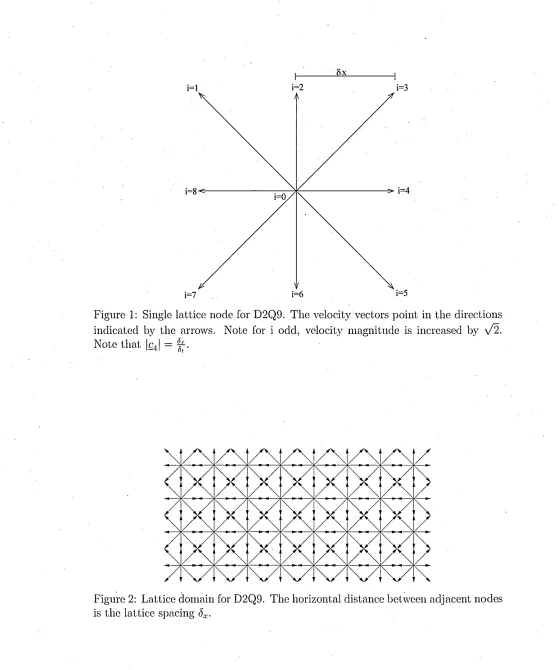
The essential idea of lattice Boltzmann is to solve this equation on a regular lattice made-up from a ‘basis’ or unit cell of discrete velocity vectors (see figure 1). This discrete velocity set c* will then define all the positions on the lattice.

The D2Q9 LBE method operates on a two dimensional (D = 2) lattice with

nine (Q = 9) possible velocity vectors. The lattice is essentially square with eight velocity vectors connecting nearest and next-nearest lattice nodes, the ninth, zero vector corresponds to the central rest node. The velocity vector direction is indexed by the quantity “i”, the velocity vectors are denoted using c{ as shown (figure 1).

Each of the nodes depicted in figure 1 are arranged on a regular lattice that

covers the simulation domain (figure 2).

The magnitude of the velocity vector is denoted as the vector population distri

bution function, fi. The vector populations (fi) are controlled by a set of governing

laws that may be used to obtain the macroscopically observable quantities of the flow.

In General LB is a directional discretization of equation (33) in velovity space:

fi (r + Ci6t , t + 6t) = / - M ) = /i( r ,0 + ^*j ( /j 0)(p,v) - / j M ) ) +'&• (34)

In equation (34) £2^- is known as the collision matrix and fi is the population of particles travelling with velocity c{ [3]. The term will be considered in greater detail in later sections, for current purposes it may be regarded as a term used to

m , L + ZSut + 6t) - m , r , t ) =

f(£ ,L + (St,t + 5t) = - f (0\ p , u ) ) .

T

(37)

i=l i=2 i=3

■5- i=4

=8

i:

i=0.

[image:37.612.0.559.30.700.2]

i=6

i=7

Figure 1: Single lattice node for D2Q9. The velocity vectors point in the directions

indicated by the arrows. Note for i odd, velocity magnitude is increased by y/2.

Note that |c4| = y1.

Figure 2: Lattice domain for D2Q9. The horizontal distance between adjacent nodes

(38)

impose an external force on the fluid such as a gravitational field. In general, the lattice fluid’s kinematic viscosity is determined by the principal eigenvalue of the

symmetric collision matrix = fyi- For the single relaxation time so-called LBGK

model Qij takes a simple form:

with the collision parameter r determining the fluid kinematic viscosity; for our

particular D2Q9 choice [3]:

where 6X is the lattice spacing see figure 1 and 5t is the time step. Note that the

lattice spacing 5x = 1 throughout. The 0 ^ or r are assumed to be known.

For the D2Q9 model of Qian and d’Humieres [4], analysed in detail by Hou et

al [27];

turn density; tpG is a “source” term, where tp is the lattice link weight, which may be used for example, to represent a uniform pressure gradient [3,28] or interfacial tension as an external force, in the case of multiple immiscible fluids [3]; all other symbols have their usual meaning [4,27].

Algorithmically, equation (37) is interpreted as a collision step (right hand side of (37)) followed by a “streaming” or “propagation” step in which the calculated value of the right hand side is moved in the direction of ci for an interval 5t to reach the next lattice node.

(35)

(36)

f j (r, t) is the “post-collision”, “pre-propagate” (see below) value of the

(39)

i 0(rest) 1 2 3 4 5 6 7 8

tp 4/9 1/9 1/36 1/9 1/36 1/9 1/36 1/9 1/36

Cix 0 1 1 0 -1 -1 -1 0 1

■ Piy 0 0 1 1 1 0 -1 -1 -1

Table 1: Definition of the D2Q9 simulation lattice link vectors, c

For all LB models the equilibrium distribution function is linear in p:

f i 0)(p,v) = p P t;1) (v • Cj) , (38)

where the second-order polynomial P^2)(v-Ci) depends upon the particular LB model

being used [3].

The principal contribution to the distribution function is the equilibrium distri bution function, which for LBGK, is defined as:

= t pp V • c_Cl (V • Ci)21

2c2 2cf

We derive the macroscopic fluid density and momentum as follows:

(39)

(40)

It will be shown below how the form of equation (39) is arrived at.

In the present context equations (39) and (40) refer to those lattice links ci and weights tp defined in Table 1 and depicted in figure 1 where the speed of sound

cs = 1/ \/3 for the D2Q9 lattice. The above choice for the equilibrium distribution function also recovers a pressure tensor:

ni°i =

\ p S a » + P'l'aV fj = f f ' c i a d p . (41) [image:39.614.16.558.31.768.2]

(40)

Continuity equations for the flow problem. It is not a trivial exercise to show that,

as we shall now see. • .

4.1.2 Chapman Enskog Expansion for Macroscopic Dynamics

Within this section I attem pt a limited but direct derivation of the hydrodynamic equations recovered from the Boltzmann equation via the Chapman Enskog expan sion. Key points arising within this derivation will be referred to in following sections notably Chapter 6.

The Chapman-Enskog [29] analysis allows us to recover the hydrodynamic equa tions from the lattice Boltzmann evolution equations. The LB equation is initially expanded to second order accuracy in space and time with relation to the Knudsen number [3], Through algebraic manipulation and scaled expansion a set of equations may be obtained at short and long distance scales and fast and slow time scales.

Working from the LBGK evolution equation we shall show how to arrive at the hydrodynamic equations and derive a system of simultaneous equations for param eters in fj;0\

We begin with the LBGK evolution equation from equation (37) that is clearly space and time discretised:

fi(x + 8tCii t + 8t) = fi(x, t) + - ( / i (0) - fi(x, t)). (42) T

Taylor expansion of equation (42) in two dimensions, retaining terms up to and including second order along with cancellation of like terms yields:

5((ci.V + ^ ) / i + § ( c i.V + ^ ) 2/i = i ( i ; (0) - / ife i)). (43)

The time and space derivatives are now Chapman Enskog expanded into parts con sisting of their long and short components, this effective expansion of the variables

(41)

formally being carried out with relation to the Knudsen number, 5. We therefore make the following expansions:

&t — fto + fidth (44)

/• = /i(0) + <5/j(1) + 52f P . (45)

Substituting the above definitions into equation (43) we obtain an expression that may subsequently be separated into first and second moments in terms of the Chap

man Enskog Knudsen number expansion parameter 5 which is set equal to 6t:

6(cj.V + dto + 59(i)(//0) + S f P + S2f P )

+^y(CjV + 9(° + JcJtiXcjV + fl(° + + 5/j® + <52/ j 2*)

= ~ l ( S f P + S2f P ) . (46)

Collecting and separately equating terms in 5 and 52 it is possible to express the first and second moments of the distribution function as;

(Ci.V + at0) / f > = - i / | 1), (47)

(ciV + dto)ri1) + dtj W + ^ {ci V + dmf f ) = - l f p , (48)

Through straightforward algebraic manipulation of equation (48) and insertion of equation (47) we can obtain a form of equation (48) that is more easily manipulated

within the analysis: <

(1

- l ) ( c i V + d t0) f } 1) + d n f l 0) = - - f F ) .

(49)

It . t

We now have a set of equations that consider the first and second moments of the

(42)

the lattice basis summation moments that are imposed on the distribution function. For the conservation of mass, Chapmann and Enskog required:

- /*:

£ i/i(">0) = 0. (50)

Similarly for momentum considerations we may follow Chapmann and Enskog:

E i/i(0)Cj = pa,

S i/ i<">°)a = 0. (51)

Taking the equation for the first moment 5o(l), equation (47) and summing on “i” and inserting the above momentum and mass conservation considerations we can show that we have produced the continuity equation with short time scale components [30]. Expressed in tensor notation, we have;

dtop + dapua = 0. (52)

Considering the second moment of o(£), equation (47) we can write the equation in tensor notation and multiply through by c^:

Xiciad J ? )cil3 + Z idtot f )cil3 = - - Z if l 1)ci0._T (53)

Using the identities expressed in equations (50) and (51), we may express equation (53) as;

ZiCiadafPcid + dtopup = 0. (54)

W ith an eye on the required emergent behaviour (see below) we require the

(43)

rium” contribution f - ° \ of the distribution function fi to have the following property;

^ ifi C-iaC-iP ~ ^sP^aP Pea'll/.3*

Substitution of (55) into (54) yields;

dtopup + dac2sp5a/3 + dapuaU(3 = 0. (56)

Through tensor algebra we can exploit the property of the Kronecker Delta function in order to change the equation subscripts and subsequently in order to expand the equation further we invoke the product rule for differentiation. Cancellation of terms may then be carried out using the continuity equation, equation (52), to transform terms within the equation. The equation resulting from these operations is:

dtoup + uadaup = -dpc2sln(p). (57)

Comparison of equation (57) with earlier work shows that our model reproduces a form of the Euler equation on short time scales. Thus far we have used the equation

containing terms of first order in “6" to recover the continuity and Euler equations

on short time scales.

We can now proceed to considerations of the longer time scale o(S2), equation

(49). Summation of equation (49) on “i” and taking into account the mass and momentum conservation constraints identified in equations (50) and (51) we have the equation;

dtlp = 0. • (58)

Multiplication of equation (58) with “5" and adding with, from the previous analysis,

(44)

recovers the continuity equation on long time scales:

dtp + da(pUa) = 0. (59)

In order to obtain further dynamics of the system we return to the o(52) equation,

equation (49). Multiplication throughout by a second velocity vector ap prior to

summation on the “i” components yields the following;

dnZif^C ip + (1 - ^ -)£ i(3(0 + CiO0a) / f % = - - S j f ci/3, (60)

It t

to which we return to in Chapter 6, note.

Using equation (51), equation (60) may be simplified (having made a substitution for the first moment of the distribution function, ./*, in conjunction with equation (47) in tensor format):

dtipup + (1 - -^)<9a2i(-T(<9<0 + CiydJf^CiaCip = 0. (61)

Through general expansion and substitution of the definitions made in equation (55) we obtain from the above a form that may be expanded further using the product rule for differentiation:

dtipup + ( i - r)da dt0c2sp5ap + updtopua + puadmup + d7E i/-°)Q7q acii0 = 0. (62)

The second and third terms contained within the square bracket in equation (62) may be expanded using definitions derived from the Euler equation on a short time scale, equation (57), giving;

dtiP^p T (^ [clySj/) CijCiaC{p -{- dtocsp5ap

—UpC^daP — UpdjpUjUa — Ua(?sdpp — UapUjdjUp] = 0. (63)

(45)

The fourth and final terms within the square bracket may now be combined using the reverse of the product rule for differentiation resulting in;

dnpup + ( i - r)a a [57Eit/-(0)ci7ciaci/3 + dtoc2sp5ap

—upc2sdap - uac2sdpp - d1puaupu1\ = 0. (64)

The final term in the square bracket of equation (64) is conventionally called the error term and is an undesirable but unavoidable occurrence within the analysis. Dropping the error term from the analysis and substituting in the continuity equation in order to remove the time derivative from the second term within the bracket, results in;

^tlPUp ~b (^ 7 " ) ^ a [ ^ 7 CsdapUa5ap

-upc2sdap - uac2dpp] = 0. (65)

The time derivative dt\pup will be incorporated naturally into the overall time deriva

tive when equations (57)and (65) are combined it is disregarded for the moment. By considering only the function contained within the square brackets we obtain a further constraint on the equilibrium distribution function required to achieve Navier-Stokes behaviour:

Ci'yCiaCiP CsâPâ^&P ^pCs^&P â^s^PP = ^PâP

Henceforth we shall also neglect the term that is quadratic in velocity. Through cal culus and general algebraic manipulation the above expression may be manipulated into a form resembling the Navier-Stokes equation [30].

(46)

certain that the steps above may be achieved. We write:

fiykQ ~ “b B(j-U§Ci§ “I- C a U§UtCj§Cit ~b

fii0

~

Aa

+

Dau5u5.

By recalling the constraints that have been applied to the equilibrium distribution function in order to recover the hydrodynamic equations in the above analysis it is possible to generate a system of simultaneous equations in A...D that allow us to determine values for the constants in the general form of the equilibrium distribution function equation. For convenience the constraints on the equilibrium distribution function we have just used are summarized again below:

^ i f i Q a = P ^ a t

^ i f i CiaCi(3 — ^sP^aP “b p U a llp ,

~b ^P&aP ”b ^ a ^ p P ) “b fcpSafi

For the lattice depicted in figure 1 (and indeed any viable LB simulation lattice) it may be shown that:

^ ^ tpCjct —

i

^ v tpCjgCjp ^2^apt i

^ ^ tpCiaCipCi^ 0,

i

^

tp Cia C i

(69)

(68)

(67)

(47)

where &2 = §, and k± = | (for the D2Q9 lattice).

Essentially the first three of the above constraints will determine the form of the

equilibrium distribution function and the value of the models speed of sound cs. The

fourth of the constraints uses the speed of sound to identify exactly the value of the constant k in equation (68) as jL Equilibrium distribution functions summations in (68) are now decomposed into separate summations of the rest link and of the short links (+) and of the long links (x). Considering the first of the constraints summarized in system (68);

— -do + 4v4i + 4^2 + BiTi+usCi§ + B^BAusCis + C iB+usUtCi8Citi

+C2£ x usUtCisCa + (D0 4Di -t- 4D2)?/2 = p. (70)

The above condition must hold for all values of fluid velocity, v. We therefore obtain

two equations governing the coefficients of the equilibrium distribution function:

Aq + 4j4i + 4^2 = Pi (71)

2 Ci + 4C2 + Dq + 4Di + 4.D2 = 0. (72)

The second of the equilibrium distribution function weighted summations in (6 8)

may now be considered;.

B*ifi Qict — B \ B U§Ci§Cia “I- BqB UftCi$Cia

~\~C\B U5'UjtCi8CitCia T C2B U§U^C{§C{iCia

+ D 0ciau2 + ADiciau2 + Cia4D2u2 = pua. (73)

(48)

the equilibrium distribution function;

2Bx + 4,B2 = p. (74)

Performing similar operations with the second and third velocity moments allows us to produce further relations between the coefficients in the equilibrium distribution function defined in (70). When considering the third q moment we force a condition on the C coefficients, namely;

2Ci - 8C2 = 0. (75)

This condition insures Gallilean invariance [31]. Making this assumption within the second q moment of the equilibrium distribution function allows us to make the following statements:

2(A\ + 2A2) = c2sp, (76)

8 C2 = p, (77)

4C*2 + 2{Di + 2D2) = 0. (78)

We can now consider the third q moment of the equilibrium distribution function in equation (68) which generates the following constraint on the coefficients of the equilibrium distribution function:

2#! - 8B2 = 0. (79)

Manipulating the third velocity moment into a form to generate the Navier-Stokes equation gives a final restriction on the equilibrium distribution function [31]:

B 2 = & . (80)

(49)

We have now produced a set of simultaneous equations that restrict the coefficients of the equilibrium distribution function in such a way as to allow us to recover con ventional hydrodynamics namely the continuity and Navier-Stokes equations from the lattice Boltzmann equation algorithm. The system of equations however is not a conventional system of equations, as it is under-determined i.e. we have a system of eight equations in ten unknowns. The system also contains subsets of equations, these subsystems may be solved exactly:

Aq +4j4i +4.A2 = p 1

2A\ +4^2 ' = c2p,

B\ +4i?2 = p 1

2 Ci +4C2+D0 +4Di +4D2 — 0,

2 C i-8 C 2 = 0 ,

8C2 = p ,

4C2 +2Di + 4D2 = 0 5

2B\ —8B2 = 0.

(81)

The subsystems contained within the set of eight equations allows the coefficients .Bi, B2, Ci and C2 to be solved completely. It is also worth noting that the B.2 coefficient determines the speed of sound c2s in the calculations. Through equation (76) the value of B2 also constrains the values of the coefficients ^4i and A2 therefore the range of “free” coefficients is somewhat restricted. We can note that the values selected for the “free variables” will effect the overall properties of the system. The choice of Aq for instance will determine the amount of rest mass contained on a

link. The selection of a large value of Aq will restrict the attainable Mach number of

(50)

i = l — 8. Having solved for A...D, the in LBGK may be written:

f i 0)(p>v ) = u p 1 -t V - C ; — . V~r~z_2c22 + ( v- Cj )2_{2 ci} (82)

4.1.3 Length and Time Scale Considerations

When considering the behaviour of momentum transfer within a fluid, as would be expected, internal friction causes the fluid distribution function to return to ther modynamic equilibrium. The momentum of the particles of the fluid and thus the information that they carry is transferred through collisions. Low density systems such as low density gases transfer information slowly as collisions between particles are rare, the length scales, viscosity and density of the simulation therefore influence the rate at which a simulation achieves its equilibrium velocity distribution. The equilibrium state of a fluid may be achieved through different processes depending on the time scales involved.

A first relaxation regime occurs when the system under consideration consists of many bodies and the time scales involved are shorter than the duration of a collision event. Due to the short time scales there must be rapid relaxation of the many body distribution function, occurring at the collision, to the single particle distribution function. In the Boltzmann regime the collisions are assumed to be instantaneous and therefore the relaxation mechanism considered in this system are ignored.

The second relaxation mode is the kinematic regime where the time scales are in the region of the duration of the time of flight between collision events; The Maxwellian equilibrium distribution is a many body ensemble average over a local region where