Comparative Study of Retinal Blood Vessel
Segmentation based on SVM and K-NN
Classification
Syed Akhter Hussain1, Deshmukh.R.R2, Osmani Mohsin3 1, 3Aditya Engineering College, Beed (MS) India -431122
2Department of Computer Science & IT, Dr. Babasaheb Ambedkar Marathwada University, Aurangabad (MS) India -431001
Abstract: Glaucoma is one of the most leading eye disease in the world it damages the optic nerve, the part of the eye which carries the images in the form of electrical signals to the brain, and leads to loss of vision. It is caused due to the enormous increase in the intraocular pressure in which rate of secretion of the ciliary body is unstable to the rate of drainage in the drainage canal. Depending on how the pressure rises, glaucoma is mainly classified as Open angle and Angle-closure glaucoma. At later stages of life, glaucoma cannot be treated due to severe damage to the optic nerve as disease prolongs, therefore, early stages of glaucoma detection are necessary.
Manually detection of glaucoma is tedious and sensitive which depends on ophthalmologist to overcome this we present retinal vessel segmentation model which is based on a discriminatively trained, fully connected conditional random field model. We used Standard segmentation priors such as a Potts model or total variation typically fail when dealing with thin and elongated structures. We conquer this complexity by using a conditional random field model with more meaningful potentials, fascinating advantage of current results enabling presumption of fully connected models almost in real-time. Parameters of the method are learned automatically using a structured output support vector machine and k-nearest neighbour, a supervised technique widely used for structured prediction in a number of machine learning applications. outcome: Our method is trained with extraordinary features, is evaluated both on publicly available data sets with quantitatively and qualitatively: DRIVE, STARE, CHASEDB1 and HRF. in addition, a quantitative comparison with respect to other strategies is included. Conclusion: The experimental results demonstrate that this approach is better then other techniques when evaluated in terms of sensitivity, F1-score, G-mean and Matthews correlation coefficient. Additionally, it was observed that the fully connected model is able to better differentiate the desired structures than the local neighborhood based approach. Significance: Results suggest that k-nn classification of this method is suitable then svm, a feature that can be exploited to contribute with other medical and biological applications.
Keywords:conditional random field, blood vessel segmentation ,fudus images ,svm,k-nn.
I. INTRODUCTION
Automated segmentation of blood vessels in retinal images is very vital in early detection and diagnosis of many eye diseases. It is an important step in screening programs for early detection. Methods for blood vessels segmentation of retinal images, according to the classification method, are divided into two groups, supervised and unsupervised methods. The development of automatic tools for the early detection of retinal diseases is valuable since they can be easily integrated in screening programs, where large numbers of images are taken from patient populations, and careful evaluation by physicians is not feasible in a reasonable time [1]. These tools are usually aided by the analysis of morphological attributes of retinal blood vessels, which provide valuable information for the diagnosis, screening, treatment and evaluation of the previously mentioned diseases [1]. In other cases, vessels need to be previously detected in order to facilitate the automation of the detection of lesions with similar intensities [2]. However, any automated analysis of the retinal vasculature requires its accurate segmentation first. In current best practice, this task is performed manually by trained experts, although this is particularly tedious and time-consuming. Furthermore, difficulties in the imaging process–such as inadequate contrast between vessels and background, and uneven background illumination–and the variability of vessel width, brightness and shape, reduce significantly the coincidence among segmentations performed by different human observers [3]. These facts motivate the development of automatic strategies for blood vessel segmentation without human intervention [1].
[8], [9], decision trees [10], [11], Gaussian mixture models [3], AdaBoost [12], among others. A trainable filter, named B-COSFIRE, was recently introduced in [13] to highlight the retinal vasculature. Though the method is not supervised in the sense of training a classifier, the strategy they follow to adjust its parameters is based on training data. By contrast, unsupervised methods are systems that are able to segment the vasculature without requiring any manual annotations, although typically at the cost of lower accuracy. In general, most of these strategies are based on applying thresholding, vessel tracking techniques [14] or region-oriented approaches–such as region growing [15]–[17] or active contours [18], [19]–after vessel enhancement. This task is performed by means of morphological operations [20], matched filter responses [21]–[22], the complex continuous wavelet transform [23], among others [24]. The method we propose in this paper belongs to the supervised category.
Conditional Random Fields (CRFs) are extensively used for image segmentation in several applications [25]–[27]. To the best of our knowledge, however, they were never applied before to blood vessel segmentation in fundus images. This is likely due to that the standard pairwise potentials, such as in a Potts model, assign a low prior to the elongated structures that comprise a vessel segmentation. This fact motivated us to introduce a novel method for blood vessel segmentation based on fully connected CRFs [25], which we extend in this article. Fully connected CRFs were previously applied in [29] and [30] for liver and brain tumor segmentation in CT and MRI, but their implications on the segmentation of two dimensional, thin structures was not previously studied. In this work we demonstrate that the dense connectivity augments the capability of the method to detect elongated structures, overcoming the original difficulty of local neighborhood based CRFs and improving results significantly. This property can potentially contribute to a number of different biological and medical applications where the segmentation of such structures is required, including automatic plant root phenotyping [31] or neuron analysis [32].
As is shown in [33], local classification leads to misclassification issues that might arise while incorporating prior knowledge about the shape of the desired structures on the learning process. CRFs are able to provide such information through the pairwise potentials. Structured Output SVM (SOSVM) has been used before to learn local neighborhood based CRFs [34], [35]. However, learning dense CRFs using SOSVMs was avoided before due to its computational intractability, since the learning method requires multiple calls to the inference algorithm during training, and the inference in dense CRFs is usually slow. We overcome this problem by making use of recent advances in efficient inference in fully connected CRFs [33].
In this paper, we complement our previous work [28] with further information and implementation details. We also modify the strategy to estimate additional parameters of the method in order to optimize its performance during training. Additionally, we extend the validation of our results with an evaluation performed both quantitatively and qualitatively on four standard and publicly available data sets (DRIVE, STARE, CHASEDB1 and HRF) to study the behaviour of the algorithm under different contexts, including images of healthy patients, containing pathologies and taken at different resolutions. According to our experiments, this method outperforms current strategies when evaluating in terms of several different quality measures.
II. METHODOLOGY
We present an broad description and evaluation of our method for blood vessel segmentation in fundus images based on a discriminatively trained, fully connected conditional random field model. Methods: Standard segmentation priors such as a Potts model or total variation usually fail when dealing with thin and elongated structures. We overcome this difficulty by using a conditional random field model with more expressive potentials, taking advantage of recent.
A. Conditional Random Fields for Vessel Segmentation
Conditional random field solves an energy minimization problem in segmentation task. In the original meaning of CRFs, images are mapped to graphs, where each pixel represents a node, and every node is connected with an edge to their neighbors according to a certain connectivity rule [26], [33], [36]. In local neighborhood based CRFs, nodes are connected following a 4 pixel neighborhood connectivity [37], while in the fully connected definition each node is assumed to be linked to every other pixel of the image [33]. We denote by y = {yi} a labeling over all pixels of the image I in the label space L = {-1, 1}, where 1 is
associated to blood vessels and -1 to any other class. A conditional random field (I, y) is characterized by the Gibbs distribution:
Where Z(I) is a normalization constant, G is the graph associated to I and CG is a set of cliques in G, each inducing a potential
[30]. This distribution states the conditional probability of a labeling y given the image I. The Gibbs energy function can be derived from this likelihood:
Thus, the maximum a posterior (MAP) labeling can be obtained by minimizing the corresponding energy:
After minimizing E(y|I), a binary segmentation of the vasculature is obtained. For notational convenience, we will skip the conditioning in the rest of the paper, and we will use to denote . Additionally, we will consider energies that decompose as summations over unary and pairwise potentials, in contrast to more general higher order potentials [38].
Given a graph G on y, its energy is obtained by summing its unary and pairwise potentials ( and , respectively):
Where Xi and fi are the unary and pairwise features, respectively. Unary potentials define a log-likelihood over the label
assignment y, and they are traditionally computed by a classifier [36]. Pairwise potentials define a similar distribution but considering only the interactions between pixels features and their labels, according to CG, which is determined by the graph
connectivity.
1) Local Neighborhood Based CRFs: Local neighborhood based CRFs (LNB-CRFs) are defined over grid graphs. Thus, in this type of model each node (pixel) is assumed to be connected by an edge to its 4-connected neighbors. The function for the pairwise potentials given the m-th pairwise feature is obtained as follows:
Where is a bandwidth that controls the relevance of the dissimilarities between pixel features? The energy of the grid based model is minimized using the min-cut/max-flow approach proposed by [37].
2) Fully Connected CRFs: In a fully connected CRF model (FC-CRF), each node of the graph is assumed to be linked to every other pixel of the image. Using these higher order potentials, the method is able to take into account not only neighboring information but also long-range interactions between pixels. This property improves the segmentation accuracy, but makes implementation of the inference process computationally expensive in general. Recently, however, Krahenbuhl and Koltun [33] have introduced an efficient inference approach under the restriction that the pairwise potentials are a linear combination of Gaussian kernels over an Euclidean feature space. This approach, which is based on taking a mean field approximation of the original CRF, is able to produce accurate segmentations in a few seconds. Pairwise kernels for the fully connected model have the following form:
Where pi and pj are the coordinate vectors of pixels i and j. Positions are included in the pairwise terms to increase the effect of
B. Learning CRFs with Structured Output SVM
Our aim is to learn a vector , where , and are the weights for the unary features, for the bias term and for the pairwise kernels, respectively. The vector w can be high-dimensional if multiple features are considered, so manual or automated adjustment using techniques such as grid search is not feasible in a reasonable time. Supervised learning of the unary potentials separately from the pairwise potentials might be an alternative, but this approach ignores the influence of the pairwise potentials on the general energy formulation, and can lead to worse results than joint learning of the weights. We therefore propose to obtain w in a supervised way, using the 1-slack formulation of the SOSVM with margin-rescaling presented in [35]. Such a discriminative training approach has shown promising results for building highly complex and accurate models in several areas, including object detection, image segmentation and computer vision applications, even for large datasets. To the best of our knowledge, however, it was never used before for the task of learning FC-CRFs.
The weights w are obtained by solving:
Where C is a regularization constant; is a slack variable shared across all the constraints
C. Features
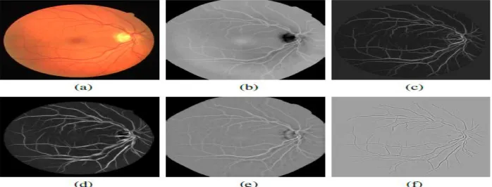
We evaluated our method using features that are widely used in the field of blood vessel segmentation in fundus images: responses to the multiscale line detectors presented by Nguyen et al. [42] and responses to 2D Gabor wavelets [5] are used to compute the unary potentials, and a vessel-enhanced image processed with the method by Zana and Klein [20] for the pairwise potentials. All features are extracted from grey scale images, obtained by taking the inverted green band of the original, RGB color image, as reported by other works [8], [13]. Additionally, due to false detections introduced by the selected features on the border of the FOV, we replicate the strategy proposed in [5] to simulate a wider aperture of the capture device. By means of this technique, false detections occurring outside the original FOV can be easily removed by multiplying the resulting image with the original FOV mask. 2D Gabor wavelets have the capability to detect oriented features and can be tuned to specific frequencies. This property is especially useful to enhance the vasculature, since blood vessels appear at different sizes and orientations. We compute this feature exactly as reported by Soares et al. [5] at different scales a. Responses of the image to this wavelet, taken at different values of a, are included as features. Fig. 1d depicts an example obtained with a = 3.
[image:4.595.124.473.611.744.2]Zana and Klein’s technique for vessel enhancement takes advantage of the fact that the vessels are linear connected, and their curvature varies smoothly along the crest line [20]. Noise of the image is first reduced by applying an opening by reconstruction operation, using linear structuring elements of length l at different angles. Afterwards, multiple top-hat morphological operations are applied using the same structuring elements, and the sum of the corresponding responses for each given angle is taken. This transformation reduces small bright noise and improves the contrast of all linear components. Structures whose curvature is linearly coherent are then detected by means of a cross-curvature evaluation, performed by applying a Laplacian of Gaussian with windows of size 7 _ 7 pixels and standard deviation 7=4. Finally, an alternating filter composed by successive application of a morphological opening, a closing and an opening is applied to remove false detections of non linear patterns on bright or dark thin irregular zones and background linear features. In the three last operations, the same linear structuring element of length l is used. We have observed that this feature is highly sensitive to uneven illumination of the fundus, degrading its ability to characterize the blood vessels effectively. In order to improve its quality we incorporated an additional preprocessing, only for this feature, where an estimated background is subtracted from the green band of the original color image.
Figure 2.Image preprocessing and unary and pairwise features examples. (a) Original color image. (b) Inverted green band after border expansion. (c) Response to Nguyen et al. line detector (l = 15). (d) Response to Soares et al. 2D Gabor wavelet at the
The background is estimated by convolving the green band with a median filter, where the size of the filter kernel is large enough to ensure that the blurred image contains no visible structures such as vessels. All features are normalized independently to zero mean and unit variance, using the mean and the standard deviation of each feature calculated on each image [5].
D. Scaling Models to Images of Different Resolution
Although the weights for the unary features and the pairwise kernels are adjusted during the learning process, system performance is still related to the capability of the features to effectively characterize vascular structure. In general, features are sensitive to their parameters, which are usually related to vessel properties such as their caliber, which is at the same time related to the image resolution. Responses to the 2D Gabor wavelet, for example, depend on the scale a. Similarly, [39]Nguyen et al. line detectors and the Zana and Klein enhancement strategy depend on the length l of the detectors or the linear structuring element, respectively. Most of these feature parameters were originally set using low resolution images, such as those in the DRIVE dataset [40]. When applying such features to higher resolution images, performance is significantly reduced if the feature extraction procedure is not proportionately scaled. Other parameters such as the angles for computing feature responses at different orientations are not influenced by changes in the resolution of the images.
A similar behavior can be expected for preprocessing parameters, e.g. the size of the median filter used to estimate the background, or the size of the aperture simulated by the border expansion. The parameter used on the pairwise potentials of the FC-CRF is also influenced by image resolution, since it weighs the pairwise interactions according to the relative distance of each pixel.
E. KNN Classifier
The KNN k-nearest neighbor’s algorithm (k-NN) is a non-parametric method used for classification and regression. In both cases, the input consists of the k closest training examples in the feature space. The output depends on whether k-NN is used for classification or regression:
1) In k-NN classification, the output is a class membership. An object is classified by a majority vote of its neighbors, with the object being assigned to the class most common among its k nearest neighbors (k is a positive integer, typically small). If k = 1, then the object is simply assigned to the class of that single nearest neighbor.
2) In k-NN regression, the output is the property value for the object. This value is the average of the values of its k nearest neighbors.
k-NN is a type of instance-based learning, or lazy learning, where the function is only approximated locally and all computation is deferred until classification. The k-NN algorithm is among the simplest of all machine learning algorithms.
Both for classification and regression, a useful technique can be used to assign weight to the contributions of the neighbors, so that the nearer neighbors contribute more to the average than the more distant ones. For example, a common weighting scheme consists in giving each neighbor a weight of 1/d, where d is the distance to the neighbor.
The neighbors are taken from a set of objects for which the class (for k-NN classification) or the object property value (for k-NN regression) is known. This can be thought of as the training set for the algorithm, though no explicit training step is required. A peculiarity of the k-NN algorithm is that it is sensitive to the local structure of the data.
a) Algorithm: The training examples are vectors in a multidimensional feature space, each with a class label. The training phase of the algorithm consists only of storing the feature vectors and class labels of the training samples. In the classification phase, k is a user-defined constant, and an unlabeled vector (a query or test point) is classified by assigning the label which is most frequent among the k training samples nearest to that query point. A commonly used distance metric for continuous variables is Euclidean distance. For discrete variables, such as for text classification, another metric can be used, such as the overlap metric (or Hamming distance). In the context of gene expression microarray data, for example, k -NN has also been employed with correlation coefficients such as Pearson and Spearman. Often, the classification accuracy of k-NN can be improved significantly if the distance metric is learned with specialized algorithms such as Large Margin Nearest Neighbor or Neighborhood components analysis. A drawback of the basic "majority voting" classification occurs when the class distribution is skewed. That is, examples of a more frequent class tend to dominate the prediction of the new example, because they tend to be common among the k nearest neighbors due to their large number. One way to overcome this problem is to weight the classification, taking into account the distance from the test point to each of its k nearest neighbors. The class (or value, in regression problems) of each of the k nearest points is multiplied by a weight proportional to the inverse of the distance from that point to the test point. Another way to overcome skew is by abstraction in data representation.
techniques (see hyper parameter optimization). The special case where the class is predicted to be the class of the closest training sample (i.e. when k = 1) is called the nearest neighbor algorithm. The accuracy of the k-NN algorithm can be severely degraded by the presence of noisy or irrelevant features, or if the feature scales are not consistent with their importance. Much research effort has been put into selecting or scaling features to improve classification. A particularly popular approach is the use of evolutionary algorithms to optimize feature scaling. Another popular approach is to scale features by the mutual information of the training data with the training classes.In binary (two class) classification problems, it is helpful to choose k to be an odd number as this avoids tied votes. One popular way of choosing the empirically optimal k in this setting is via bootstrap method.
c) The weighted nearest neighbor classifier: The k-nearest neighbor classifier can be viewed as assigning the k nearest neighbors a weight and all others 0 weight. This can be generalized to weight nearest neighbor classifiers. That is, where
the ith nearest neighbor is assigned a weight , with . An analogous result on the strong consistency of weighted nearest neighbour classifiers also holds. Let denote the weighted nearest classifier with weights . Subject to regularity conditions on to class distributions the excess risk has the following asymptotic expansion
d) Properties:k-NN is a special case of a variable-bandwidth, kernel density "balloon" estimator with a uniform kernel. The naive version of the algorithm is easy to implement by computing the distances from the test example to all stored examples, but it is computationally intensive for large training sets. Using an approximate nearest neighbor search algorithm makes
k-NN computationally tractable even for large data sets. Many nearest neighbor search algorithms have been proposed over the years; these generally seek to reduce the number of distance evaluations actually performed. k-NN has some strong consistency results. As the amount of data approaches infinity, the two-class k-NN algorithm is guaranteed to yield an error rate no worse than twice the Bayes error rate (the minimum achievable error rate given the distribution of the data). Various improvements to the k-NN speed are possible by using proximity graphs.
III.RESULTS AND DISSCUSION
To better understand our system we have enlist some steps how system works
A. Input image
B. Convert input image to gray scale
C. Estimate the mean component in the gray scale image
D. Subtract it from the background image for estimation
E. Check for change in orientation by applying bicubic filter
F. Convolve the filter for fitting the orientation
G. Evaluate the highest filter response
H. Evaluate the eigen values by normalizing the image
I. Enhance the image using local edge features
J. Evaluate the threshold to binarize the image
K. Go for vessel segmentation by complementing the extracted edge regions using the threshold factor
L. Evaluate the energy content in the image using entropy factor.
M. Load the database saved .mat files to extract the database features
N. Train the database using svm classifier
O. Apply prediction for the testdata using svm for the trainer dataset.
P. Evaluate the cross validation points and evaluate the performance of classifier
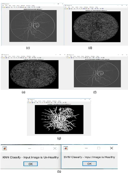
Q. Repeat steps 14-16 using KNN classifier and evaluate the performance. Output of system given as follows
(c) (d)
(e) (f)
(g)
[image:7.595.109.518.81.635.2](h)
Figure 3.segmentation and classification results(a) input image (b)gray scale image(c)eigen enhanced image(d)wavelet enhanced result(e)local enhanced result (f)background normalize image(g)vessel segmentation result(h) svm and k-nn
classification result
1) Evaluation Metrics: Results were analyzed quantitatively by comparing our segmentations with the gold standard labelings provided on each data set. Seven different measurements were obtained, all of them in terms of the number of true positives TP, true negatives TN, false positives FP and false negatives FN, and considering only the pixels inside the FOV:
,
Table: 1 performance analysis for svm Table: 2 performance analysis for k-nn
0.00% 10.00% 20.00% 30.00% 40.00% 50.00% 60.00% 70.00% 80.00% 90.00% 100.00%
Sensitivity(svm)
specificity(svm)
accuracy(svm)
Sensitivity(knn)
specificity(knn)
accuracy(knn)
Graph: 1 performance measurement for svm and k-nn classification
IV.CONCLUSIONS
In this work, we have presented a comparative study of classification for both SVM and k-NN in our work first at all we go for segmentation for ROI and feature extraction here we used FC-CRF By means of features extracted from the images and fully connected pairwise potentials, this approach is able to reconstruct the retinal vasculature much more precisely than using only the unary potentials or a local neighborhood based CRF. By means of features extracted from the images and fully connected pairwise potentials, this approach is able to reconstruct the retinal vasculature much more precisely than using only the unary potentials or a local neighborhood based CRF. The capability of the dense potentials to reconstruct elongated structures can potentially benefit other biological and medical applications. Our system shows knn is most superior then svm in terms of specivity, sensitivity and accuracy
Images Sensitivity specificity accuracy Result
01-Test 93.3333% 90.9091% 85.6% unhealthy
02-Test 93.3333% 91.8182% 87.2% unhealthy
03-Test 93.3333% 90.9091% 84% unhealthy
04-Test 93.3333% 90.9091% 85.6% unhealthy
05-Test 93.3333% 90.9091% 85.6% unhealthy
06-Test 93.3333% 90% 84.8% unhealthy
07-Test 93.3333% 90.9091% 84% unhealthy
08-Test 93.3333% 90% 84.8% unhealthy
09-Test 93.3333% 88.1818% 83.2% unhealthy
10-Test 93.3333% 91.8182% 86.4% unhealthy
11-Test 93.3333% 90.9091% 86.4% unhealthy
12-Test 93.3333% 90.9091% 85.6% unhealthy
Image01-L 93.3333% 89.0909% 84% healthy
Images Sensitivity specificity accuracy results
01-Test 46.6667% 78.1818% 80% unhealthy
02-Test 53.3333% 78.1818% 80% unhealthy
03-Test 33.3333% 77.2727% 79.2% unhealthy
04-Test 46.6667% 78.1818% 80% unhealthy
05-Test 46.6667% 78.1818% 80% unhealthy
06-Test 46.6667% 78.1818% 80% unhealthy
07-Test 33.3333% 78.1818% 80% unhealthy
08-Test 46.6667% 78.1818% 80% unhealthy
09-Test 46.6667% 78.1818% 80% unhealthy
10-Test 46.6667% 78.1818% 80% unhealthy
11-Test 53.3333% 78.1818% 80% unhealthy
12-Test 46.6667% 78.1818% 80% unhealthy
REFERENCES
[1] M. D. Abr`amoff et al., “Retinal imaging and image analysis,” Biomedical Engineering, IEEE Reviews in, vol. 3, pp. 169–208, 2010.
[2] M. Esmaeili et al., “A new curvelet transform based method for extraction of red lesions in digital color retinal images,” in Image Processing (ICIP), 2010 17th IEEE International Conference on. IEEE, 2010, pp. 4093–4096.
[3] P. Dai et al., “A new approach to segment both main and peripheral retinal vessels based on gray-voting and gaussian mixture model,” PloS one, vol. 10,
no. 6, p. e0127748, 2015
[4] M. Niemeijer et al., “Comparative study of retinal vessel segmentation methods on a new publicly available database,” in Medical Imaging 2004.
International Society for Optics and Photonics, 2004, pp. 648– 656.
[5] J. V. Soares et al., “Retinal vessel segmentation using the 2-D Gabor wavelet and supervised classification,” Medical Imaging, IEEE Transactions on, vol.
25, no. 9, 2006.
[6] L. Xu and S. Luo, “A novel method for blood vessel detection from retinal images,” Biomedical engineering online, vol. 9, no. 1, p. 14, 2010.
[7] X. You et al., “Segmentation of retinal blood vessels using the radial projection and semi-supervised approach,” Pattern Recognition, vol. 44, no. 10,
2011.
[8] D. Mar´ın et al., “A new supervised method for blood vessel segmentation in retinal images by using gray-level and moment invariants-based features,”
Medical Imaging, IEEE Transactions on, vol. 30, no. 1, pp. 146–158, 2011.
[9] R. Vega et al., “Retinal vessel extraction using lattice neural networks with dendritic processing,” Computers in biology and medicine, vol. 58, pp. 20–30,
2015.
[10] M. M. Fraz et al., “An ensemble classification-based approach applied to retinal blood vessel segmentation,” Biomedical Engineering, IEEE Transactions
on, vol. 59, no. 9, pp. 2538–2548, 2012.
[11] M. M. Fraz et al., “Delineation of blood vessels in pediatric retinal images using decision trees-based ensemble classification,” International journal of
computer assisted radiology and surgery, vol. 9, no. 5, pp. 795–811, 2014.
[12] C. A. Lupascu et al., “Fabc: retinal vessel segmentation using adaboost,” Information Technology in Biomedicine, IEEE Transactions on, vol. 14, no. 5,
pp. 1267–1274, 2010.
[13] G. Azzopardi et al., “Trainable cosfire filters for vessel delineation with application to retinal images,” Medical image analysis, vol. 19, no. 1, pp. 46–57,
2015
[14] Y. Yin et al., “Automatic segmentation and measurement of vasculature in retinal fundus images using probabilistic formulation,” Computational and
mathematical methods in medicine, vol. 2013, 2013.
[15] M. M. Fraz et al., “Retinal vessel extraction using first-order derivative of gaussian and morphological processing,” in Advances in Visual Computing.
Springer, 2011, pp. 410–420.
[16] M. M. Fraz et al., “Application of morphological bit planes in retinal blood vessel extraction,” Journal of digital imaging, vol. 26, no. 2, pp. 274–286,
2013
[17] S. Roychowdhury et al., “Iterative vessel segmentation of fundus images,” Biomedical Engineering, IEEE Transactions on, vol. 62, no. 7, pp. 1738–1749,
2015
[18] B. Al-Diri et al., “An active contour model for segmenting and measuring retinal vessels,” Medical Imaging, IEEE Transactions on, vol. 28, no. 9, pp.
1488–1497, 2009.
[19] Y. Zhao et al., “Automated vessel segmentation using infinite perimeter active contour model with hybrid region information with application to retina
images,” Medical Imaging, IEEE Transactions on, 2015
[20] F. Zana and J.-C. Klein, “Segmentation of vessel-like patterns using mathematical morphology and curvature evaluation,” Image Processing, IEEE
Transactions on, vol. 10, no. 7, pp. 1010–1019, 2001.
[21] G. B. Kande et al., “Unsupervised fuzzy based vessel segmentation in pathological digital fundus images,” Journal of medical systems, vol. 34, no. 5, pp.
849–858, 2010
[22] T. Chakraborti et al., “A self-adaptive matched filter for retinal blood vessel detection,” Machine Vision and Applications, vol. 26, no. 1, pp. 55–68, 2014.
[23] A. Fathi and A. R. Naghsh-Nilchi, “Automatic wavelet-based retinal blood vessels segmentation and vessel diameter estimation,” Biomedical Signal
Processing and Control, vol. 8, no. 1, pp. 71–80, 2013
[24] A. Soltanipour et al., “Vessel centerlines extraction from fundus fluorescein angiogram based on hessian analysis of directional curvelet subbands,” in Acoustics, Speech and Signal Processing (ICASSP), 2013 IEEE International Conference on. IEEE, 2013, pp. 1070–1074.
[25] X. He et al., “Multiscale conditional random fields for image labeling,” in Computer Vision and Pattern Recognition, 2004. CVPR 2004. Proceedings of
the 2004 IEEE Computer Society Conference on, vol. 2. IEEE, 2004, pp. II–695.
[26] S. Kumar and M. Hebert, “Discriminative random fields,” Int. J. Comput. Vision, vol. 68, no. 2, pp. 179–201, Jun. 2006.
[27] S. Z. Li, Markov Random Field Modeling in Image Analysis, 3rd ed. Springer, 2009
[28] J. I. Orlando and M. Blaschko, “Learning fully-connected CRFs for blood vessel segmentation in retinal images,” in MICCAI 2014, LNCS, P. Golland, C.
Barillot, J. Hornegger, and R. Howe, Eds. Springer, 2014, vol. 8149, pp. 634–641.
[29] S. Kadoury et al., “Higher-order crf tumor segmentation with discriminant manifold potentials,” in Medical Image Computing and Computer- Assisted
Intervention–MICCAI 2013. Springer, 2013, pp. 719–726.
[30] S. Kadoury et al., “Metastatic liver tumour segmentation from discriminant grassmannian manifolds,” Physics in Medicine and Biology, vol. 60, no. 16, p.
6459, 2015
[31] F. Fiorani and U. Schurr, “Future scenarios for plant phenotyping,” Annual review of plant biology, vol. 64, pp. 267–291, 2013.
[32] M. Helmstaedter, “Cellular-resolution connectomics: challenges of dense neural circuit reconstruction,” Nature methods, vol. 10, no. 6, pp. 501– 507,
2013.
[33] P. Kr¨ahenb¨uhl and V. Koltun, “Efficient inference in fully connected CRFs with Gaussian edge potentials,” in Advances in Neural Information
Processing Systems, 2012, pp. 109–117
[34] Ioannis Tsochantaridis et al.,”Large Margin Methods for Structured and Interdependent Output Variables”2005,pp.1453-1484.
[35] Ioannis Tsochantaridis et al.,”cutting-plane training of structural SVMs”machine learning,vol.77,no.1pp.27-59,2009
[36] John Lafferty et .al”Conditional Random Fields: Probabilistic Models for Segmenting and Labeling Sequence Data” in Proceedings of the 18th
[37] Y. Boykov et .al “An experimental comparison of min-cut/max- flow algorithms for energy minimization in vision ”IEEE Transactions on Pattern Analysis and Machine Intelligence Volume: 26 , Issue: 9 , Sept. 2004
[38] Nikos Komodakis et .al”MRF Energy Minimization and Beyond via Dual Decomposition” IEEE Transactions on Pattern Analysis and Machine
Intelligence Volume: 33 , Issue: 3 , March 2011
[39] Uyen T.V.Nguyen et .al ”An effective retinal blood vessel segmentation method using multi-scale line detection ” pattern recognition volume46 issue 3,
March 2013, Pages 703-715
[40] Joes Staal et.al “Ridge-Based Vessel Segmentation in Color Images of the Retina” IEEE TRANSACTIONS ON MEDICAL IMAGING , VOL. 23, NO.