Stanford’s Graph based Neural Dependency Parser at the CoNLL 2017 Shared Task

Stanford’s Graph-based Neural Dependency Parser at the CoNLL 2017

Shared Task

Timothy Dozat Stanford University

[email protected]

Peng Qi Stanford University

[email protected]

Christopher D. Manning Stanford University

[email protected]

Abstract

This paper describes the neural depen-dency parser submitted by Stanford to the CoNLL 2017 Shared Task on parsing Uni-versal Dependencies. Our system uses relatively simple LSTM networks to pro-duce part of speech tags and labeled de-pendency parses from segmented and tok-enized sequences of words. In order to ad-dress the rare word problem that abounds in languages with complex morphology, we include a character-based word rep-resentation that uses an LSTM to pro-duce embeddings from sequences of char-acters. Our system was ranked first ac-cording to all five relevant metrics for the system: UPOS tagging (93.09%), XPOS tagging (82.27%), unlabeled attachment score (81.30%), labeled attachment score (76.30%), and content word labeled at-tachment score (72.57%).

1 Introduction

In this paper, we describe Stanford’s approach to tackling the CoNLL 2017 shared task on Univer-sal Dependency parsing (Nivre et al., 2016; Ze-man et al.,2017;Nivre et al.,2017b,a). Our sys-tem builds on the deep biaffine neural dependency parser presented by Dozat and Manning (2017), which uses a well-tuned LSTM network to pro-duce vector representations for each word, then uses those vector representations in novel biaffine classifiers to predict the head token of each depen-dent and the class of the resulting edge. In order to adapt it to the wide variety of different treebanks in Universal Dependencies, we make two note-worthy extensions to the system: first, we incor-porate a word representation built up from char-acter sequences using an LSTM, theorizing that

this should improve the model’s ability to adapt to rare or unknown words in languages with rich morphology; second, we train our own taggers for the treebanks using nearly identical architecture to the one used for parsing, in order to capitalize on potential improvements in part of speech tag qual-ity over baseline or off-the-shelf taggers. This ap-proach gets state-of-the-art results on the macro average of the shared task datasets according to all five POS tagging and attachment accuracy metrics. One noteworthy feature of our approach is its relative simplicity. It uses a single tagger/parser pair per language, trained on only words and tags; thus we refrain from taking advantage of ensem-bling, lemmas, or morphological features, any one of which could potentially push accuracy even higher.

2 Architecture

2.1 Deep biaffine parser

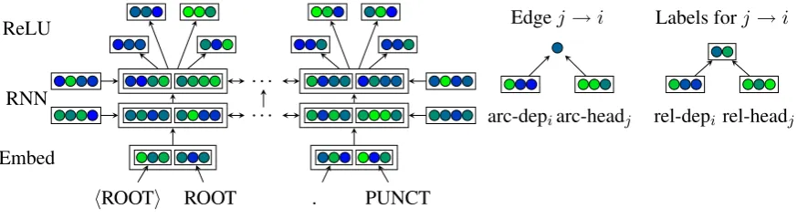
The basic architecture of our approach follows that of Dozat and Manning (2017), which is closely related to Kiperwasser and Goldberg (2016), the first neural graph-based (McDonald et al., 2005) parser.1 _{InDozat and Manning’s2017parser, the}

input to the model is a sequence of tokens and their part of speech tags, which is then put through a multilayer bidirectional LSTM network. The out-put state of the final LSTM layer (which excludes the cell state) is then fed through four separate ReLU layers, producing four specialized vector representations: one for the word as a dependent seeking its head; one for the word as a head seek-ing all its dependents; another for the word as a de-pendent deciding on its label; and a fourth for the word as head deciding on the labels of its

depen-1_{For other neural graph-based parsers, cf.Cheng et al.} (2016);Hashimoto et al.(2016);Zhang et al.(2016)

. . . . . .

hROOTi ROOT . PUNCT

RNN

Embed ReLU

arc-depiarc-headj rel-depi rel-headj

Labels forj→i

Edgej →i

Figure 1: The architecture of our parser. Arrows indicate structural dependence, but not necessarily trainable parameters.

dents.2_{These vectors are then used in two biaffine}

classifiers: the first computes a score for each pair of tokens, with the highest score for a given to-ken indicating that toto-ken’s most probable head; the second computes a score for each label for a given token/head pair, with the highest score represent-ing the most probable label for the arc from the head to the dependent. This is shown graphically in Figure1.

Put formally, given a sequence of nword em-beddings (to be described in more detail in Section 2.2)(v(₁word), . . . ,v(nword))andntag embeddings (v₁(tag), . . . ,vn(tag)), we concatenate each pair

to-gether and feed the result into a BiLSTM with ini-tial stater0:3

xi =v(iword)⊕v(itag) (1)

ri =BiLSTM r0,(x1, . . . ,xn)_i (2)

hi,ci =split(ri) (3)

We then produce four distinct vectors from each recurrent hidden state hi (without the recurrent

cell stateci) using ReLU perceptron layers:

h(_iarc-dep) =MLP(arc-dep)_(h

i) (4)

h(_iarc-head) =MLP(arc-head)(hi) (5)

h(_irel-dep) =MLP(rel-dep)(hi) (6)

h(_irel-head) =MLP(rel-head)_(h

i) (7)

In order to produce a predictiony_i0(arc)for token

i, we use a biaffine classifier involving the(arc) 2_{Interestingly, other researchers have found similar} ap-proaches to be beneficial for other tasks; cf.Reed and de Fre-itas(2016);Miller et al.(2016);Daniluk et al.(2017)

3_{We adopt the convention of using lowercase italics for} scalars, lowercase bold for vectors, uppercase italics for ma-trices, and uppercase bold for tensors. We maintain this con-vention when indexing and stacking; soaiis theith vector of matrixA, and matrixAis the stack of all vectorsai.

hidden vectors:

s(_iarc)=H(arc-head)W(arc)h(_iarc-dep) (8)

+H(arc-head)b>(arc) y_i0(arc)= arg max

j s

(arc)

ij (9)

Note first the similarity between line8and a tra-ditional affine classifier of the form Wh + b, with each ofW andb first being transformed by

H(arc-head)_{. Note also that both terms of the}

bi-affine layer have intuitive interpretations: the first relates to the probability of wordjbeing the head of wordigiven the information in bothh(arc)

vec-tors (for example, the probability of word i de-pending on word j given that word i is the and wordjiscat); the second relates to the probability of wordjbeing the head of wordigiven only the information in the head’s vector (for example, the probability of wordidepending on word j given that wordj isthe, which should be very small no matter what wordiis).

After deciding on a heady0

i for word i, we use

another biaffine transformation—this time involv-ing the (rel) hidden vectors—to produce a pre-dicted label:

s(_irel)=h>(rel-head)

y0_i(arc) U(rel)h

(rel-dep)

i (10)

+W(rel) h_i(rel-dep)⊕h(rel-head)

y0_i(arc)

+b(rel) y0_i(rel)= arg max

j s

(rel)

ij (11)

Again, each term in line10 has an intutive inter-pretation: the first term relates to the probability of observing a label given the information in both h(rel) _{vectors (e.g. the probability of the labeldet}

i n f e r RNN

Embed Attn/Final Cell

Linear

Char

Token word2vec Char

Tag

UPOS XPOS Embed

Sum

Word

Embed Sum

Figure 2: The architecture of our embedding model. Arrows indicate structural dependence, but not necessarily trainable parameters.

eitherh(rel)_{vector (e.g. the probability of the label}

detgiven that wordiistheor that wordj iscat); the last relates to the prior probability of observing a label.

We jointly train these two biaffine classifiers by optimizing the sum of their softmax cross-entropy losses. At test time, we ensure the tree is well-formed by iteratively identifying and fixing cycles for each proposed root and selecting the one with the highest score, which is both simple and suffi-cient for our purposes.4

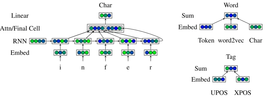
2.2 Character-level model

Dozat and Manning(2017) represented words as the sum of a pretrained vector5_{and a holistic word}

embedding for frequent words. However, that ap-proach seems insufficient for languages with rich morphology; so we add a third representation built up from sequences of characters. Each character is given a trainable vector embedding, and each sequence of character embeddings is fed into a unidirectional LSTM. However, the LSTM pro-duces asequenceof recurrent states(r1, . . . ,rn),

which we need to convert into a single vector. The simplest approach is to take the last one—which would represent a summary of all the information aggregated one character at a time—and linearly transform it to the desired dimensionality. An-other approach, suggested byCao and Rei(2016), is to use attention over the hidden states, and then 4_{Although in the future we intend to implement than the} Chu-Liu/Edmonds algorithm for nonprojective MST parsing (Chu and Liu,1965;Edmonds,1967)

5_{We use the provided CoNLL vectors trained on} word2vec (Mikolov et al.,2013); for Gothic, which had no provided vector embeddings, we used Facebook’s FastText vectors (Bojanowski et al.,2016)

trasform the resulting context vector to the desired size; in theory, this should both allow the model to learn morpheme information more easily by at-tending more closely to the LSTM output at mor-pheme boundaries. We choose to combine both approaches, using the hidden states for attention and the cell state for summarizing, shown in Fig-ure2.

That is, given a sequence of n character em-beddings and an initial stater0 for the LSTM, we

each embedding into an LSTM as before, extract-ing hidden and cell states:

ri=LSTM r0,(v1(char), . . . ,v(nchar))

i

(12) hi,ci=split(ri) (13)

We then compute linear attention over the stack of hidden vectors H and concatenate it to the final cell state:

a=softmax Hw(attn) (14)

˜h=H>_{a (15)}

ˆv=W ˜h⊕cn (16)

In this way we use the hidden states for attention and the cell state as a final summary vector.

2.3 POS tagger

The final piece of our system is a separately-trained part of speech tagger. The architecture for the tagger is almost identical to that of the parser (and shares fundamental properties with other neural taggers; cf.Ling et al.(2015);Plank et al.(2016))—it uses a BiLSTM over word vec-tors (using the tripartite representation from Sec-tion 2.2), then uses ReLU layers to produce one vector representation for each type of tag.

Thus we use a BiLSTM, as with the parser ar-chitecture:

ri=BiLSTM r0,(v1(word), . . . ,v(nword))_i

(17)

hi,ci=split(ri) (18)

And we use affine classifiers for each type of tag, which we add together for the parser:

h(_ipos) =MLP(pos)_(h

i) (19)

s_i(pos) =Wh_i(pos)+b(pos) (20)

y_i0(pos) = arg max j s

(pos)

ij (21)

The tag classifiers are trained jointly using cross-entropy losses that are summed together during optimization, but the tagger is trained indepen-dently from the parser.

3 Training details

Our model largely adopts the same hyperparam-eter configuration laid out by Dozat and Man-ning (2017), with a few exceptions. The parser uses three BiLSTM layers with 100-dimensional word and tag embeddings and 200-dimensional re-current states (in each direction); the arc classi-fier uses 400-dimensional head/dependent vector states and the label classifier uses 100-dimensional ones; we drop word and tag embeddings inde-pendently with 33% probability;6 _{we use}

same-mask dropout (Gal and Ghahramani,2015) in the LSTM, ReLU layers, and classifiers, dropping in-put and recurrent connections with 33% proba-bility; and we optimize with Adam (Kingma and Ba, 2014), setting the learning rate to 2e−3 _and

β1 = β2 = .9. We train models for up to 30,000

training steps (where one step/iteration is a single minibatch with approximately 5,000 tokens), at 6_{When only one is dropped, we scale the other by a factor} of two

first saving the model every 100 steps if fewer than 1,000 iterations have passed, and afterwards only saving if validation accuracy increases (or training accuracy for languages with no validation data). When 5,000 training steps pass without improving accuracy, we terminate training.

For the character model, we use 100-dimensional uncased character embeddings with 400-dimensional recurrent states. We don’t drop characters but do include 33% dropout in the LSTM and attention connections.

In the tagger we use nearly identical settings, with a few exceptions: the BiLSTM is only two layers deep, we increase the dropout between re-current connections to 50%, and we use cased character embeddings.

Our approach for dealing with the surprise lan-guages was to train delexicalized “language fam-ily” parsers with the same architecture detailed in Section2.1on UDPipe v1.1 (Straka et al.,2016)’s UPOS tags with no word-level information. For Buryat (Altaic), we used as input the training datasets for Turkish, Uyghur, Kazakh, Korean, and Japanese; for Kurmanji (Indo-Iranian), we used Persian, Urdu, and Hindi; for North S´ami (Uralic), we used Finnish, Finnish-FTB, Estonian, and Hungarian; and for Upper Sorbian (Slavic), we used Bulgarian, Czech, Old Church Slavonic, Pol-ish, Russian, Russian-SynTagRus, Slovak, Slove-nian, Slovenian-SST, and Ukrainian.

There’s substantial variability in training and testing speed across treebanks, but on an NVidia Titan X GPU the models train at 100 to 1000 sen-tences/sec and test at 1000 to 5000 sensen-tences/sec. Even without GPU acceleration a tagger or parser can be run on an entire test treebank in ten to twenty seconds. By far the greatest runtime over-head comes not from the model itself, but from reading in the large matrices of pretrained em-beddings, which can take several minutes. A full run over the 81 test sets on the TIRA virtual ma-chine (Potthast et al.,2014) takes about 16 hours, but when parallelized on faster machines it can be done in under an hour.

4 Results

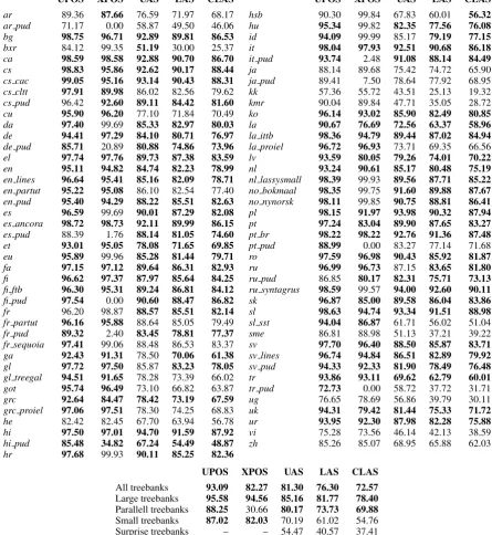
UPOS XPOS UAS LAS CLAS ar 89.36 87.66 76.59 71.97 68.17 ar pud 71.17 0.00 58.87 49.50 46.06 bg 98.75 96.71 92.89 89.81 86.53 bxr 84.12 99.35 51.19 30.00 25.37 ca 98.59 98.58 92.88 90.70 86.70 cs 98.83 95.86 92.62 90.17 88.44 cs cac 99.05 95.16 93.14 90.43 88.31 cs cltt 97.91 89.98 86.02 82.56 79.62 cs pud 96.42 92.60 89.11 84.42 81.60 cu 95.90 96.20 77.10 71.84 70.49 da 97.40 99.69 85.33 82.97 80.03 de 94.41 97.29 84.10 80.71 76.97 de pud 85.71 20.89 80.88 74.86 73.96 el 97.74 97.76 89.73 87.38 83.59 en 95.11 94.82 84.74 82.23 78.99 en lines 96.64 95.41 85.16 82.09 78.71 en partut 95.22 95.08 86.10 82.54 77.40 en pud 95.40 94.29 88.22 85.51 82.63 es 96.59 99.69 90.01 87.29 82.08 es ancora 98.72 98.73 92.11 89.99 86.15 es pud 88.39 1.76 88.14 81.05 74.60 et 93.01 95.05 78.08 71.65 69.85 eu 95.89 99.96 85.28 81.44 79.71 fa 97.15 97.12 89.64 86.31 82.93 fi 96.62 97.37 87.97 85.64 84.25 fi ftb 96.30 95.31 89.24 86.81 84.12 fi pud 97.54 0.00 90.60 88.47 86.82 fr 96.20 98.87 88.57 85.51 82.14 fr partut 96.16 95.88 88.64 85.05 79.49 fr pud 89.32 2.40 83.45 78.81 77.37 fr sequoia 97.41 99.06 88.48 86.53 83.37 ga 92.43 91.31 78.50 70.06 61.38 gl 97.72 97.50 85.87 83.23 78.05 gl treegal 94.51 91.65 78.28 73.39 66.02 got 95.74 96.49 73.10 66.82 63.87 grc 92.64 84.47 78.42 73.19 67.59 grc proiel 97.06 97.51 78.30 74.25 68.83 he 82.42 82.45 67.70 63.94 56.78 hi 97.50 97.01 94.70 91.59 87.92 hi pud 85.48 34.82 67.24 54.49 48.87 hr 97.68 99.93 90.11 85.25 82.36

UPOS XPOS UAS LAS CLAS

hsb 90.30 99.84 67.83 60.01 56.32

hu 95.34 99.82 82.35 77.56 76.08 id 94.09 99.99 85.17 79.19 77.15 it 98.04 97.93 92.51 90.68 86.18 it pud 93.74 2.48 91.08 88.14 84.49

ja 88.14 89.68 75.42 74.72 65.90

ja pud 89.41 7.50 78.64 77.92 68.95

kk 57.36 55.72 43.51 25.13 19.32

kmr 90.04 89.84 47.71 35.05 28.72

ko 96.14 93.02 85.90 82.49 80.85 la 90.67 76.69 72.56 63.37 58.96 la ittb 98.36 94.79 89.44 87.02 84.94 la proiel 96.72 96.93 73.71 69.35 66.56 lv 93.59 80.05 79.26 74.01 70.22 nl 93.24 90.61 85.17 80.48 75.19 nl lassysmall 98.39 99.93 89.56 87.71 85.22 no bokmaal 98.35 99.75 91.60 89.88 87.67 no nynorsk 98.11 99.85 90.75 88.81 86.41 pl 98.15 91.97 93.98 90.32 87.94 pt 97.24 83.04 89.90 87.65 83.27 pt br 98.22 98.22 92.76 91.36 87.48 pt pud 88.99 0.00 83.27 77.14 71.68 ro 97.59 96.98 90.43 85.92 81.87 ru 96.99 96.73 87.15 83.65 81.80 ru pud 86.85 80.17 82.31 75.71 73.13 ru syntagrus 98.59 99.57 94.00 92.60 90.11 sk 96.87 85.00 89.58 86.04 83.86 sl 98.63 94.74 93.34 91.51 88.98 sl sst 94.04 86.87 61.71 56.02 51.04

sme 86.81 88.98 51.13 37.21 39.22

sv 97.70 96.40 88.50 85.87 83.71 sv lines 96.74 94.84 86.51 82.89 79.92 sv pud 94.33 92.33 81.90 78.49 76.48 tr 93.86 93.11 69.62 62.79 60.01 tr pud 72.73 0.00 58.72 37.72 31.71

ug 76.65 78.69 56.86 39.79 30.11

uk 94.31 79.42 81.44 75.33 71.72 ur 93.95 92.30 87.98 82.28 75.88

vi 75.28 73.56 46.14 42.13 38.59

zh 85.26 85.07 68.95 65.88 62.03

UPOS XPOS UAS LAS CLAS All treebanks 93.09 82.27 81.30 76.30 72.57 Large treebanks 95.58 94.56 85.16 81.77 78.40 Parallell treebanks 88.25 30.66 80.17 73.73 69.88 Small treebanks 87.02 82.03 70.19 61.02 54.76 Surprise treebanks – – 54.47 40.57 37.41

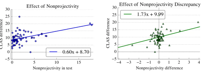
0 5 10 15 Nonprojectivity in test −5

0 5 10 15 20 25 30

CLAS difference

Effect of Nonprojectivity

0.60x + 8.70

(a) Difference in CLAS between our parser and UDPipe v1.1 as a function of the nonprojectivity of the test set

−4 −3 −2 −1 0 1 2 3 4

Nonprojectivity difference −5

0 5 10 15 20 25 30

CLAS difference

Effect of Nonprojectivity Discrepancy

1.73x + 9.99

(b) Difference in CLAS between our parser and UDPipe v1.1 as a function of the difference between the nonprojectivity of the test and training sets

Figure 3: How the percent of nonprojective arcs in the training and test set influence accuracy of our graph-based and a transition-based parser

and content labeled attachment score. Our system achieves the highest aggregated score on all five of these metrics in the shared task. Below we explore where our model does particularly well, and where it can be improved. We choose to evaluate on CLAS performance because we feel it more accu-rately reflects model performance, being a princi-pled extension of the common practice of remov-ing punctuation from evalution. We also exclude surprise languages from the following analyses.

One small point to that end is that our sys-tem assumes tokenization and segmentation has already been done; we therefore trained on gold segmentation and evaluated using the segmenta-tion provided by UDPipe. For most treebanks this was easily sufficient, but for Vietnamese, Chi-nese, JapaChi-nese, and Arabic, UDPipe’s lower per-formance at segmenting or tokenizing was corre-lated with a relatively large gap between CLAS and gold-aligned CLAS. Because our model re-ports comparable numbers for nearly all other tree-banks, we take this to mean that alignment errors propagated through the system into parsing errors.

4.1 Nonprojectivity

In Universal Dependencies, unlike many other popular benchmarks, several treebanks have a large fraction of crossing dependencies, so any competitive system will need to be able to produce nonprojective arcs. One of the most frequently used approaches for producing fully nonprojec-tive parsers in transition-based systems is to add

the swap action (Nivre, 2009). This makes any arbitrary nonprojective arc possible, but increases the number of transition steps required to produce that arc. One valid concern is that this might bias the model toward producing projective arcs; in our graph-based system, by contrast, there’s little rea-son to think nonprojective arcs should be harder to predict than projective ones. Here we aim to ex-plore how the fraction of nonprojective arcs in a treebank affects the performance of the two types of systems.

103 ₁₀4 ₁₀5 ₁₀6 Training size

−20 −15 −10 −5 0 5 10

CLAS difference

Effect of Training Size

2.59log₁₀(x) - 11.89

Figure 4: Performance difference between our model and the highest-performing model other than ours as a function of log training data size

This remains significant even when outliers7 _are

excluded(p < 0.05). To the extent that UDPipe represents a typical nonprojective transition-based parser, our results suggest that a graph-based ap-proach is better suited to parsing UD treebanks that have significant syntactic freedom or com-plexity than a transition-based one.

Predicting crossing arcs requires more opera-tions (and therefore more long-term planning on behalf of the parser) when using the swap fea-ture in a transition-based system, but in our graph-based system they can be predicted as easily as projective arcs. One might hypothesize that be-cause of this, a transition-based swapping sys-tem would need to see more examples of cross-ing dependencies than a graph-based system in or-der to generalize well. The data shown in Figure 3bsupport this hypothesis: we computed the dif-ference between the projectivity of each test and training set, and used this as the fixed effect in another mixed effects model with data size, mor-phological complexity, and train/test nonprojec-tivity as random effects. We find that when the training set has drastically fewer crossing depen-dencies than the test set, the graph-based model achieves relatively higher accuracy; but when the transition-based parser can train on many cross-ing arcs, the models are closer in performance (p < 0.001), even when excluding the same out-liers (p < 0.05). This suggests that the graph-based approach learns and generalizes crossing dependencies more efficiently than the

transition-7_{Korean (top); Ancient Greek, Latin (right)}

0 2 4 6 8 10

UPOS difference 0

2 4 6 8

CLAS difference

Effect of Tagger Improvement

0.35x + 0.75

Figure 5: Performance difference between a ver-sion of our model trained on our own predicted tags and a version trained on UDPipe v1.1 tags as a function of the performance difference between our taggers and the UDPipe taggers

based approach, although this again comes with the assumption that UDPipe’s parser is represen-tative of most transition-basedswapping parsers when it comes to producing nonprojective parses.

4.2 Data size

We use the same hyperparameter configuration for all datasets, regardless of how much training data there is for that treebank, which means we may have overfit to small training datasets or underfit to large ones. To test this, we computed the treebank difference between the test CLAS per-formance of our model and that of the highest-performing model other than ours, and plotted that ratio against the log training data size in Figure 4. We fit the differences to another mixed ef-fects regression model with train/test projectivity and morphological complexity set as random ef-fects, finding that our system on average tends to do relatively better on larger datasets compared to other approaches and worse on smaller ones (p < 0.001). When the outliers are excluded,8

this tendency is still significant(p <0.001). This suggests that our model is overfitting to smaller datasets, and that increasing regularization or de-creasing model capacity may improve accuracy for lower-resource languages.

−1 0 1 2 3 4 5 6 7 8 CLAS difference

0.0 0.1 0.2 0.3 0.4

0.5 Own Tagger vs. No Tagger

−8 −6 −4 −2 0 2 4

CLAS difference 0.0

0.1 0.2 0.3 0.4 0.5

0.6 UDPipe Tagger vs. No Tagger

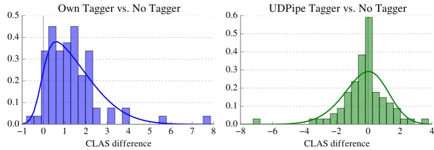
Figure 6: Performance difference between parsers using our taggers and parsers without tags (left) and between parsers using UDPipe v1.1’s tags and parsers without tags (right), with both histograms fit to skew normal distributions

5 Ablation Studies 5.1 POS Tagger

We chose to train our parsers on our own pre-dicted tags instead of using provided taggers; here we aim to justify that strategy empirically with an ablation study. We trained another set of parsers with otherwise identical hyperparameter settings using the baseline tags provided by UDPipe v1.1, and computed the difference in CLAS between our reported models and the new ones. We also computed the difference in UPOS accuracy be-tween UDPipe v1.1’s taggers and our own. In Figure 5, we plot how the difference in tagger quality affects the CLAS of the parser, making two noteworthy observations. The first is that the performance difference between the set of mod-els trained on our own tags is statistically signif-icantly better than the performance of the models trained on UDPipe tags according to a Wilcoxon test(p < 0.001). The second is that this can be explained by the improvement of our tagger over UDPipe v1.1, again accounting for dataset size, nonprojectivity, and morphology in a mixed ef-fects model(p < 0.001). This suggests that im-proving upstream tagger performance is an effec-tive way of improving downstream parser accu-racy. We also examined the effect of training size on the difference in parser performance, finding no significant correlation(p >0.05).

The approach laid out in this paper uses one neural network to tag the sequences of tokens, and a second neural network to produce a parse from the tokens and tags. One might ask to what

extent the tagger network is actually necessary, for a number of reasons: presumably whatever predictive patterns it learns from the token se-quences would also be learnable by the parser net-work; errors by the tagger are likely to be propa-gated by the parser; andBallesteros et al. (2015) found that POS tags are drastically less impor-tant for character-based parsers. In order to ex-amine how useful the POS tag information is to our character-based system, we trained an addi-tional set of parsers without UPOS or XPOS in-put, comparing them to the other two, with the differences graphed in Figure6. We find that the variant with no POS tag input is likewise signif-icantly worse than our reported model according to a Wilcoxon test (p < 0.001), but not statisti-cally different from the one trained with UDPipe tags(p >0.05). This suggests that predicted POS tags are still useful for achieving maximal parsing accuracy in our system, provided the tagger’s per-formance is sufficiently high.

5.2 Character model

0.50 0.55 0.60 0.65 0.70 0.75 0.80 0.85 0.90 Heaps' coefficient

−2 0 2 4 6 8 10

CLAS difference

Effect of Morphological Complexity on Parser

7.57x - 4.42

0.50 0.55 0.60 0.65 0.70 0.75 0.80 0.85 0.90 Heaps' coefficient

−2 0 2 4 6 8 10 12 14 16

UPOS difference

Effect of Morphological Complexity on Tagger

14.37x - 8.34

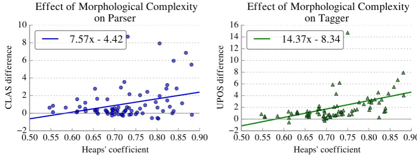
Figure 7: Performance difference between our character-based approach and a pure token-based ap-proach for parsing (left) and tagging (right) as a function of approximated morphological complexity

(for maximal comparability, we use the origi-nal character-based taggers for the token-based parsers). As morphological complexity increases, the difference between the models should increase as well.

The basis of our approach to quantifying mor-phological complexity will be the assumption that in a morphologically complex language, the ra-tio between the size of the vocabulary |V(X)_{| of}

a corpus to the size of the corpus|X|will be rel-atively high, because the same lemma may occur with many different forms; but in a morphologi-cally simplex language, that ratio will be smaller, because a given lemma will normally appear with only a few forms. Assuming both languages have the same number of lemmas, the vocabulary size of the complex language will then be larger. The most principled way of modeling this intuition is through Heaps’ law (Herdan,1960;Heaps,1978) in Equation22, which says that the log vocabulary size increases linearly in the log corpus size.

log(|V(X)|) =wlog(|X|) +b (22) We can take advantage of Heaps’ law directly in approximating morphological complexity. Mor-phologically richer languages should increase the size of their vocabulary at a faster rate as the cor-pus size grows, because a new token being added to the corpus has a higher probability of having a previously observed lemma with a previously unobserved morphological form, thereby increas-ing the vocabulary size; in a morphologically sim-plex language, previously observed lemmas are unlikely to have many morphological forms that could increase |V|. Therefore, we would expect

the parameter w of Equation 22 to be higher for languages with rich morphology. We computed this value for each treebank, and the results gen-erally align with our intuition (although not with-out some variation, attributable to domain and dataset size): Hindi and Urdu—which have sig-nificant allomorphy—are among the lowest, hav-ingw = .555and.585respectively; English and Vietnamese have.631and.661; Spanish and Por-tuguese have.7and.704; and Finnish, Estonian, and Hungarian have some of the highest, at.806,

.822, and.846.

Thus we use the coefficientwin Equation22as our metric for morphological richness, and plot the difference between models trained with character-level word embeddings and token-character-level word em-beddings against this value in Figure 7. First we perform a Wilcoxon signed rank test, finding that the difference between the two approaches is sta-tistically significant for the taggers(p < 0.001) and parsers (p < 0.001). Then we fit a mixed effects model to the data with treebank size and training/test projectivity as random effects, finding that the character-level approach tends to signifi-cantly improve performance more as complexity grows both for parsing(p < 0.005)and tagging (p < 0.001).9 _{This indicates that incorporating}

subword information into UD parsing models is a promising way to improve performance on lan-guages with significant morphology.

6 Conclusion

In this paper we describe our relatively simple neural system for parsing that achieved state-of-the-art performance on the 2017 CoNLL Shared Task on UD parsing without utilizing lemmas, morphological features, or ensembling. The sys-tem uses BiLSTM networks for tagging and pars-ing, and includes character-level word representa-tions in addition to token-level ones. We also ex-amined what can be learned more generally from our model’s performance. We explore the rel-ative performance of nonprojective graph-based and transition-based architectures on this task, finding evidence that modern graph-based parsers might be better at producing nonprojective arcs (with some caveats). Additionally, our network performs better when there’s an abundance of data, suggesting that more regularization could improve accuracy on lower-resource languages.

We also sought to quantitatively justify the ad-ditional complexity of our system. We consid-ered how important the POS tagger is to the sys-tem, comparing the downstream performance of parsers using our tagger, the baseline tagger, and no tagger at all. We find that our tagger beats both baselines significantly, whereas the two base-lines don’t statistically differ from each other, in-dicating that POS tags can help our system but must be sufficiently accurate. The character-based approach was found to significantly boost perfor-mance on languages that scored high on our met-ric for morphological complexity—both for pars-ing and taggpars-ing—suggestpars-ing that constructpars-ing to-ken representation from subtoto-ken information is effective for capturing the influence of morphol-ogy on syntax, and the na¨ıve approach of using only holistic word embeddings is insufficient. Our success at the shared task demonstrates that a well-tuned, straightforward neural approach to parsing and tagging can get state-of-the-art performance for datasets with a wide variety of syntactic prop-erties.

References

Miguel Ballesteros, Chris Dyer, and Noah A Smith. 2015. Improved transition-based parsing by model-ing characters instead of words with lstms. EMNLP .

Piotr Bojanowski, Edouard Grave, Armand Joulin, and Tomas Mikolov. 2016. Enriching word vectors with subword information. EMNLP.

Kris Cao and Marek Rei. 2016. A joint model for word embedding and word morphology. ACL 2016 page 18.

Hao Cheng, Hao Fang, Xiaodong He, Jianfeng Gao, and Li Deng. 2016. Bi-directional attention with agreement for dependency parsing. EMNLP 2016 .

Yoeng-Jin Chu and Tseng-Hong Liu. 1965. On short-est arborescence of a directed graph.Scientia Sinica 14(10):1396.

Michal Daniluk, Tim Rockt¨aschel, Johannes Welbl, and Sebastian Riedel. 2017. Frustratingly short at-tention spans in neural language modeling. ICLR 2017.

Timothy Dozat and Christopher D. Manning. 2017. Deep biaffine attention for neural dependency pars-ing.ICLR 2017.

Jack Edmonds. 1967. Optimum branchings. Journal of Research of the national Bureau of Standards B 71(4):233–240.

Ronald Aylmer Fisher. 1930. The genetical theory of natural selection: a complete variorum edition. Ox-ford University Press.

Yarin Gal and Zoubin Ghahramani. 2015. Dropout as a bayesian approximation: Representing model un-certainty in deep learning. International Conference on Machine Learning.

Jarrod D Hadfield. 2010. Mcmc methods for multi-response generalized linear mixed models: The MCMCglmm R package.Journal of Statistical Soft-ware33(2):1–22. http://www.jstatsoft.org/v33/i02/. Kazuma Hashimoto, Caiming Xiong, Yoshimasa

Tsu-ruoka, and Richard Socher. 2016. A joint many-task model: Growing a neural network for multiple nlp tasks.arXiv preprint arXiv:1611.01587.

Harold Stanley Heaps. 1978. Information retrieval: Computational and theoretical aspects. Academic Press, Inc.

Gustav Herdan. 1960. Type-token mathematics, vol-ume 4. Mouton.

Diederik Kingma and Jimmy Ba. 2014. Adam: A method for stochastic optimization. International Conference on Learning Representations.

Eliyahu Kiperwasser and Yoav Goldberg. 2016. Sim-ple and accurate dependency parsing using bidi-rectional LSTM feature representations. Transac-tions of the Association for Computational Linguis-tics4:313–327.

Ryan McDonald, Fernando Pereira, Kiril Ribarov, and Jan Hajiˇc. 2005. Non-projective dependency pars-ing uspars-ing spannpars-ing tree algorithms. InProceedings of the conference on Human Language Technology and Empirical Methods in Natural Language Pro-cessing. Association for Computational Linguistics, pages 523–530.

Tomas Mikolov, Kai Chen, Greg Corrado, and Jeffrey Dean. 2013. Efficient estimation of word represen-tations in vector space. International Conference on Learning Representations.

Alexander H. Miller, Adam Fisch, Jesse Dodge, Amir-Hossein Karimi, Antoine Bordes, and Jason We-ston. 2016. Key-value memory networks for directly reading documents. In ACL 2016. pages 1400– 1409.

Joakim Nivre. 2009. Non-projective dependency pars-ing in expected linear time. In Proceedings of the Joint Conference of the 47th Annual Meeting of the ACL and the 4th International Joint Conference on Natural Language Processing of the AFNLP: Volume 1-Volume 1. Association for Computational Linguistics, pages 351–359.

Joakim Nivre, ˇZeljko Agi´c, Lars Ahrenberg, et al. 2017a. Universal dependencies 2.0 CoNLL 2017 shared task development and test data. LIN-DAT/CLARIN digital library at the Institute of For-mal and Applied Linguistics, Charles University. http://hdl.handle.net/11234/1-2184.

Joakim Nivre, Marie-Catherine de Marneffe, Filip Gin-ter, Yoav Goldberg, Jan Hajiˇc, Christopher Man-ning, Ryan McDonald, Slav Petrov, Sampo Pyysalo, Natalia Silveira, Reut Tsarfaty, and Daniel Zeman. 2016. Universal Dependencies v1: A multilingual treebank collection. InProceedings of the 10th In-ternational Conference on Language Resources and Evaluation (LREC 2016). European Language Re-sources Association, Portoro, Slovenia, pages 1659– 1666.

Joakim Nivre et al. 2017b. Universal Dependencies 2.0. LINDAT/CLARIN digital library at the Insti-tute of Formal and Applied Linguistics, Charles Uni-versity, Prague, http://hdl.handle.net/ 11234/1-1983. http://hdl.handle.net/11234/1-1983.

Barbara Plank, Anders Søgaard, and Yoav Goldberg. 2016. Multilingual part-of-speech tagging with bidirectional long short-term memory models and auxiliary loss. ACL.

Martin Potthast, Tim Gollub, Francisco Rangel, Paolo Rosso, Efstathios Stamatatos, and Benno Stein. 2014. Improving the reproducibility of PAN’s shared tasks: Plagiarism detection, author iden-tification, and author profiling. In Evangelos Kanoulas, Mihai Lupu, Paul Clough, Mark Sander-son, Mark Hall, Allan Hanbury, and Elaine Toms,

editors, Information Access Evaluation meets Mul-tilinguality, Multimodality, and Visualization. 5th International Conference of the CLEF Initiative (CLEF 14). Springer, Berlin Heidelberg New York, pages 268–299. https://doi.org/10.1007/978-3-319-11382-1 22.

Scott E. Reed and Nando de Freitas. 2016. Neural programmer-interpreters. ICLR 2016.

Milan Straka, Jan Hajic, Jana Strakov´a, and Jan Ha-jic jr. 2015. Parsing universal dependency treebanks using neural networks and search-based oracle. In International Workshop on Treebanks and Linguis-tic Theories (TLT14). page 208.

Milan Straka, Jan Hajiˇc, and Jana Strakov´a. 2016. UD-Pipe: trainable pipeline for processing CoNLL-U files performing tokenization, morphological anal-ysis, POS tagging and parsing. In Proceedings of the 10th International Conference on Language Resources and Evaluation (LREC 2016). European Language Resources Association, Portoro, Slovenia. Daniel Zeman, Martin Popel, Milan Straka, Jan Hajiˇc, Joakim Nivre, Filip Ginter, Juhani Luotolahti, Sampo Pyysalo, Slav Petrov, Martin Potthast, Fran-cis Tyers, Elena Badmaeva, Memduh G¨okırmak, Anna Nedoluzhko, Silvie Cinkov´a, Jan Hajiˇc jr., Jaroslava Hlav´aˇcov´a, V´aclava Kettnerov´a, Zdeˇnka Ureˇsov´a, Jenna Kanerva, Stina Ojala, Anna Mis-sil¨a, Christopher Manning, Sebastian Schuster, Siva Reddy, Dima Taji, Nizar Habash, Herman Leung, Marie-Catherine de Marneffe, Manuela Sanguinetti, Maria Simi, Hiroshi Kanayama, Valeria de Paiva, Kira Droganova, Hˇector Mart´ınez Alonso, Hans Uszkoreit, Vivien Macketanz, Aljoscha Burchardt, Kim Harris, Katrin Marheinecke, Georg Rehm, Tolga Kayadelen, Mohammed Attia, Ali Elkahky, Zhuoran Yu, Emily Pitler, Saran Lertpradit, Michael Mandl, Jesse Kirchner, Hector Fernandez Alcalde, Jana Strnadova, Esha Banerjee, Ruli Manurung, An-tonio Stella, Atsuko Shimada, Sookyoung Kwak, Gustavo Mendonc¸a, Tatiana Lando, Rattima Nitis-aroj, and Josie Li. 2017. CoNLL 2017 Shared Task: Multilingual Parsing from Raw Text to Universal Dependencies. InProceedings of the CoNLL 2017 Shared Task: Multilingual Parsing from Raw Text to Universal Dependencies. Association for Computa-tional Linguistics.