Probabilistic Grammars: Sample
Complexity and Hardness of Learning
Shay B. Cohen
∗ Columbia UniversityNoah A. Smith
∗∗Carnegie Mellon University
Probabilistic grammars are generative statistical models that are useful for compositional and sequential structures. They are used ubiquitously in computational linguistics. We present a framework, reminiscent of structural risk minimization, for empirical risk minimization of prob-abilistic grammars using the log-loss. We derive sample complexity bounds in this framework that apply both to the supervised setting and the unsupervised setting. By making assumptions about the underlying distribution that are appropriate for natural language scenarios, we are able to derive distribution-dependent sample complexity bounds for probabilistic grammars. We also give simple algorithms for carrying out empirical risk minimization using this framework in both the supervised and unsupervised settings. In the unsupervised case, we show that the problem of minimizing empirical risk is NP-hard. We therefore suggest an approximate algorithm, similar to expectation-maximization, to minimize the empirical risk.
1.Introduction
Learning from data is central to contemporary computational linguistics. It is in com-mon in such learning to estimate a model in a parametric family using the maximum likelihood principle. This principle applies in the supervised case (i.e., using anno-tated data) as well as semisupervised and unsupervised settings (i.e., using unan-notated data). Probabilistic grammars constitute a range of such parametric families we can estimate (e.g., hidden Markov models, probabilistic context-free grammars). These parametric families are used in diverse NLP problems ranging from syntactic and morphological processing to applications like information extraction, question answering, and machine translation.
Estimation of probabilistic grammars, in many cases, indeed starts with the prin-ciple of maximum likelihood estimation (MLE). In the supervised case, and with traditional parametrizations based on multinomial distributions, MLE amounts to
∗ Department of Computer Science, Columbia University, New York, NY 10027, United States.
E-mail:[email protected]. This research was completed while the first author was at Carnegie Mellon University.
∗∗ School of Computer Science, Carnegie Mellon University, Pittsburgh, PA 15213, United States. E-mail:[email protected].
normalization of rule frequencies as they are observed in data. In the unsupervised case, on the other hand, algorithms such as expectation-maximization are available. MLE is attractive because it offers statistical consistency if some conditions are met (i.e., if the data are distributed according to a distribution in the family, then we will discover the correct parameters if sufficient data is available). In addition, under some conditions it is also an unbiased estimator.
An issue that has been far less explored in the computational linguistics literature is the sample complexityof MLE. Here, we are interested in quantifying the number of samples required to accurately learn a probabilistic grammar either in a supervised or in an unsupervised way. If bounds on the requisite number of samples (known as “sample complexity bounds”) are sufficiently tight, then they may offer guidance to learner performance, given various amounts of data and a wide range of parametric families. Being able to reason analytically about the amount of data to annotate, and the relative gains in moving to a more restricted parametric family, could offer practical advantages to language engineers.
We note that grammar learning has been studied in formal settings as a problem of grammatical inference—learning the structure of a grammar or an automaton (Angluin 1987; Clark and Thollard 2004; de la Higuera 2005; Clark, Eyraud, and Habrard 2008, among others). Our setting in this article is different. We assume that we have a fixed grammar, and our goal is to estimate its parameters. This approach has shown great empirical success, both in the supervised (Collins 2003; Charniak and Johnson 2005) and the unsupervised (Carroll and Charniak 1992; Pereira and Schabes 1992; Klein and Manning 2004; Cohen and Smith 2010a) settings. There has also been some discus-sion of sample complexity bounds for statistical parsing models, in a distribution-free setting (Collins 2004). The distribution-free setting, however, is not ideal for analysis of natural language, as it has to account for pathological cases of distributions that generate data.
We develop a framework for deriving sample complexity bounds using the max-imum likelihood principle for probabilistic grammars in a distribution-dependent setting. Distribution dependency is introduced here by making empirically justified assumptions about the distributions that generate the data. Our framework uses and significantly extends ideas that have been introduced for deriving sample complexity bounds for probabilistic graphical models (Dasgupta 1997). Maximum likelihood esti-mation is put in the empirical risk minimization framework (Vapnik 1998) with the loss function being the log-loss. Following that, we develop a set of learning theoretic tools to explore rates of estimation convergence for probabilistic grammars. We also develop algorithms for performing empirical risk minimization.
These also focus on learning the structure of finite state machines. As mentioned earlier, in our setting we assume that the grammar is fixed, and that our goal is to estimate its parameters.
We note an important connection to an earlier study about the learnability of probabilistic automata and hidden Markov models by Abe and Warmuth (1992). In that study, the authors provided positive results for the sample complexity for learning probabilistic automata—they showed that a polynomial sample is sufficient for MLE. We demonstrate positive results for the more general class of probabilistic grammars which goes beyond probabilistic automata. Abe and Warmuth also showed that the problem of finding or even approximating the maximum likelihood solution for a two-state probabilistic automaton with an alphabet of an arbitrary size is hard. Even though these results extend to probabilistic grammars to some extent, we provide a novel proof that illustrates the NP-hardness of identifying the maximum likelihood solution for probabilistic grammars in the specific framework of “proper approximations” that we define in this article. Whereas Abe and Warmuth show that the problem of maximum likelihood maximization for two-state HMMs is not approximable within a certain factor in time polynomial in the alphabet and the length of the observed sequence, we show that there is no polynomial algorithm (in the length of the observed strings) that identifies the maximum likelihood estimator in our framework. In our reduction, from 3-SAT to the problem of maximum likelihood estimation, the alphabet used is binary and the grammar size is proportional to the length of the formula. In Abe and Warmuth, the alphabet size varies, and the number of states is two.
This article proceeds as follows. In Section 2 we review the background necessary from Vapnik’s (1988) empirical risk minimization framework. This framework is re-duced to maximum likelihood estimation when a specific loss function is used: the log-loss.1There are some shortcomings in using the empirical risk minimization framework in its simplest form. In its simplest form, the ERM framework isdistribution-free, which means that we make no assumptions about the distribution that generated the data. Naively attempting to apply the ERM framework to probabilistic grammars in the distribution-free setting does not lead to the desired sample complexity bounds. The reason for this is that the log-loss diverges whenever small probabilities are allocated in the learned hypothesis to structures or strings that have a rather large probability in the probability distribution that generates the data. With a distribution-free assumption, therefore, we would have to give treatment to distributions that are unlikely to be true for natural language data (e.g., where some extremely long sentences are very probable).
To correct for this, we move to an analysis in a distribution-dependent setting, by presenting a set of assumptions about the distribution that generates the data. In Sec-tion 3 we discuss probabilistic grammars in a general way and introduce assumpSec-tions about the true distribution that are reasonable when our data come from natural lan-guage examples. It is important to note that this distribution need not be a probabilistic grammar.
The next step we take, in Section 4, isapproximatingthe set of probabilistic grammars over which we maximize likelihood. This is again required in order to overcome the divergence of the log-loss for probabilities that are very small. Our approximations are
based on bounded approximationsthat have been used for deriving sample complexity bounds for graphical models in a distribution-free setting (Dasgupta 1997).
Our approximations have two important properties: They are, by themselves, prob-abilistic grammars from the family we are interested in estimating, and they become a tighter approximation around the family of probabilistic grammars we are interested in estimating as more samples are available.
Moving to the distribution-dependent setting and defining proper approximations enables us to derive sample complexity bounds. In Section 5 we present the sample complexity results for both the supervised and unsupervised cases. A question that lingers at this point is whether it is computationally feasible to maximize likelihood in our framework even when given enough samples.
In Section 6, we describe algorithms we use to estimate probabilistic grammars in our framework, when given access to the required number of samples. We show that in the supervised case, we can indeed maximize likelihood in our approximation framework using a simple algorithm. For the unsupervised case, however, we show that maximizing likelihood is NP-hard. This fact is related to a notion known in the learning theory literature as inherent unpredictability (Kearns and Vazirani 1994): Accurate learning is computationally hard even with enough samples. To overcome this difficulty, we adapt the expectation-maximization algorithm (Dempster, Laird, and Rubin 1977) to approximately maximize likelihood (or minimize log-loss) in the unsupervised case with proper approximations.
In Section 7 we discuss some related ideas. These include the failure of an alter-native kind of distributional assumption and connections to regularization by maxi-mum a posteriori estimation with Dirichlet priors. Longer proofs are included in the appendices. A table of notation that is used throughout is included as Table D.1 in AppendixD.
This article builds on two earlier papers. In Cohen and Smith (2010b) we presented the main sample complexity results described here; the present article includes signifi-cant extensions, a deeper analysis of our distributional assumptions, and a discussion of variants of these assumptions, as well as related work, such as that about the Tsybakov noise condition. In Cohen and Smith (2010c) we proved NP-hardness for unsupervised parameter estimation of probalistic context-free grammars (PCFGs) (without approxi-mate families). The present article uses a similar type of proof to achieve results adapted to empirical risk minimization in our approximation framework.
2.Empirical Risk Minimization and Maximum Likelihood Estimation
In order to estimatep as accurately as possible using q(x,z), we are interested in minimizing thelog-loss, that is, in findingqopt, from a fixed family of distributionsQ
(also called “the concept space”), such that
qopt=argmin q∈Q
Ep
−logq=argmin
q∈Q
− x,z
p(x,z) logq(x,z) (1)
Note that ifp∈Q, then this quantity achieves the minimum whenqopt=p, in which case the value of the log-loss is the entropy ofp. Indeed, more generally, this optimization is equivalent to findingqsuch that it minimizes the KL divergence fromptoq.
Becausep is unknown, we cannot hope to minimize the log-loss directly. Given a set of examples (x1,z1),. . ., (xn,zn), however, there is a natural candidate, the empirical
distribution ˜pn, for use in Equation (1) instead ofp, defined as:
˜
pn(x,z)=n−1 n
i=1
I{(x,z)=(xi,zi)}
where I{(x,z)=(xi,zi)} is 1 if (x,z)=(xi,zi) and 0 otherwise.2 We then set up the
problem as the problem ofempirical risk minimization(ERM), that is, trying to findq such that
q∗=argmin
q∈Q
Ep˜n
−logq (2)
=argmin
q∈Q
−n−1 n
i=1
logq(xi,zi)
=argmax
q∈Q n−1
n
i=1
logq(xi,zi) (3)
Equation (3) immediately shows that minimizing empirical risk using the log-loss is equivalent to the maximizing likelihood, which is a common statistical principle used for estimating a probabilistic grammar in computational linguistics (Charniak 1993; Manning and Sch ¨utze 1999).3
As mentioned earlier, our goal is to estimate the probability distribution pwhile quantifying how accurate our estimate is. One way to quantify the estimation accuracy is by bounding theexcess risk, which is defined as
Ep(q;Q)=Ep(q)Ep
−logq−min
q∈QEp
−logq (4)
We are interested in bounding the excess risk for q∗, Ep(q∗). The excess risk is
reduced to KL divergence betweenp andqif p∈Q, because in this case the quantity minq∈QE
−logqis minimized withq=p, and equals the entropy ofp. In a typical
2 We note that ˜pnitself is a random variable, because it depends on the sample drawn fromp.
case, where we do not necessarily havep∈Q, then the excess risk ofqis bounded from above by the KL divergence betweenpandq.
We can bound the excess risk by showing the double-sided convergence of the empirical processRn(Q), defined as follows:
Rn(Q)sup q∈Q
Ep˜
n
−logq−Ep
−logq→0 (5)
asn→ ∞. For any >0, if, for large enoughnit holds that
sup
q∈Q
Ep˜
n
−logq−Ep
−logq< (6)
(with high probability), then we can “sandwich” the following quantities:
Ep
−logqopt
≤Ep
−logq∗ (7)
≤Ep˜n
−logq∗+
≤Ep˜n
−logqopt+
≤Ep
−logqopt
+2 (8)
where the inequalities come from the fact that qopt minimizes the expected risk
Ep
−logqforq∈Q, andq∗ minimizes the empirical riskEp˜n
−logqforq∈Q. The consequence of Equations (7) and (8) is that the expected risk ofq∗is at most 2away from the expected risk ofqopt, and as a result, we find the excess riskEp(q∗), for large
enoughn, is smaller than 2. Intuitively, this means that, under a large sample,q∗does not give much worse results thanqoptunder the criterion of the log-loss.
Unfortunately, the regularity conditions which are required for the convergence of Rn(Q) do not hold because the log-loss can be unbounded. This means that a
modifi-cation is required for the empirical process in a way that will actually guarantee some kind of convergence. We give a treatment to this in the next section.
We note that all discussion of convergence in this section has been about conver-gencein probability. For example, we want Equation (6) to hold with high probability— for most samples of sizen. We will make this notion more rigorous in Section 2.2.
2.1 Empirical Risk Minimization and Structural Risk Minimization Methods
It has been noted in the literature (Vapnik 1998; Koltchinskii 2006) that often the classQ is too complexfor empirical risk minimization using a fixed number of data points. It is therefore desirable in these cases to create a family of subclasses {Qα|α∈A}
that have increasing complexity. The more data we have, the more complex our Qα
can be for empirical risk minimization. Structural risk minimization (Vapnik 1998) and the method of sieves (Grenander 1981) are examples of methods that adopt such an approach. Structural risk minimization, for example, can be represented in many cases as a penalization of the empirical risk method, using a regularization term.
Rn(Q). Because grammars can define probability distributions over infinitely many
discrete outcomes, probabilities can be arbitrarily small and log-loss can be arbitrarily large.
To solve this issue with the complexity ofQ, we define in Section 4 a series of approx-imations{Qn|n∈N}for probabilistic grammars such that
nQn=Q. Our framework
for empirical risk minimization is then set up to minimize the empirical risk with respect toQn, wherenis the number of samples we draw for the learner:
q∗n=argmin
q∈Qn Ep˜n
−logq (9)
We are then interested in the convergence of the empirical process
Rn(Qn)= sup q∈Qn
Ep˜
n
−logq−Ep
−logq (10)
In Section 4 we show that the minimizerq∗nis anasymptoticempirical risk minimizer (in our specific framework), which means thatEp
−logq∗n→Ep
−logq∗. Because we havenQn=Q, the implication of having asymptotic empirical risk minimization
is that we haveEp(q∗n;Qn)→Ep(q∗;Q).
2.2 Sample Complexity Bounds
Knowing that we are interested in the convergence ofRn(Qn)=supq∈Qn|Ep˜n
−logq− Ep
−logq|, a natural question to ask is: “At what rate does this empirical process converge?”
Because the quantityRn(Qn) is a random variable, we need to give a probabilistic treatment to its convergence. More specifically, we ask the question that is typically asked when learnability is considered (Vapnik 1998): “How many samplesn are re-quired so that with probability 1−δwe have Rn(Qn)< ?” Bounds on this number
of samples are also called “sample complexity bounds,” and in a distribution-free setting they are described as a functionN(,δ,Q), independent of the distributionpthat generates the data.
A complete distribution-free setting is not appropriate for analyzing natural lan-guage. This setting poses technical difficulties with the convergence ofRn(Qn) and needs
to take into account pathological cases that can be ruled out in natural language data. Instead, we will make assumptions aboutp, parametrize these assumptions in several ways, and then calculate sample complexity bounds of the formN(,δ,Q,p), where the dependence on the distribution is expressed as dependence on the parameters in the assumptions aboutp.
The learning setting, then, can be described as follows. The user decides on a level of accuracy () which the learning algorithm has to reach with confidence (1−δ). Then, N(,δ,Q,p) samples are drawn from p and presented to the learning algorithm. The learning algorithm then returns an hypothesis according to Equation (9).
3.Probabilistic Grammars
process. Hidden Markov models (HMMs), for example, can be understood as a random walk through a probabilistic finite-state network, with an output symbol sampled at each state. PCFGs generate phrase-structure trees by recursively rewriting nonterminal symbols as sequences of “child” symbols (each itself either a nonterminal symbol or a terminal symbol analogous to the emissions of an HMM).
Each step or emission of an HMM and each rewriting operation of a PCFG is conditionally independent of the others given a single structural element (one HMM or PCFG state); this Markov property permits efficient inference over derivations given a string.
In general, a probabilistic grammarG,θdefines the joint probability of a stringx and a grammatical derivationz:
q(x,z|θ,G)=
K
k=1 Nk
i=1
θψk,ik,i(x,z)=exp
K
k=1 Nk
i=1
ψk,i(x,z) logθk,i (11)
where ψk,i is a function that “counts” the number of times the kth distribution’s ith event occurs in the derivation. The parameters θ are a collection of K multi-nomials θ1,. . .,θK, the kth of which includes Nk competing events. If we let θk= θk,1,. . .,θk,N
k, eachθk,iis a probability, such that
∀k,∀i, θk,i≥0
∀k,
Nk
i=1
θk,i=1
We denote byΘGthis parameter space forθ. The grammarGdictates the support of q in Equation (11). As is often the case in probabilistic modeling, there are differ-ent ways to carve up the random variables. We can think of x and z as correlated structure variables (often x is known ifz is known), or the derivation event counts ψ(x,z)=ψk,i(x,z)1≤k≤K,1≤i≤N
k as an integer-vector random variable. In this article, we assume that x is always a deterministic function of z, so we use the distribution p(z) interchangeably withp(x,z).
Note that there may be many derivations z for a given string x—perhaps even infinitely many in some kinds of grammars. For HMMs, there are three kinds of multi-nomials: a starting state multinomial, a transition multinomial per state and an emission multinomial per state. In that caseK=2s+1, wheresis the number of states. The value of Nk depends on whether the kth multinomial is the starting state multinomial (in
which case Nk=s), transition multinomial (Nk=s), or emission multinomial (Nk=t,
with t being the number of symbols in the HMM). For PCFGs, each multinomial among the K multinomials corresponds to a set of Nk context-free rules headed by
the same nonterminal. The parameterθk,iis then the probability of theith rule for the kth nonterminal.
We assume thatGdenotes a fixed grammar, such as a context-free or regular gram-mar. We let N=Kk=1Nk denote the total number of derivation event types. We use D(G) to denote the set of all possible derivations ofG. We defineDx(G)={z∈D(G)|
yield(z)=x}. We use deg(G) to denote the “degree” ofG, i.e., deg(G)=maxkNk. We
let|x|denote the length of the stringx, and|z|=Kk=1Nk
i=1ψk,i(z) denote the “length”
Going back to the notation in Section 2,Qwould be a collection of probabilistic grammars, parametrized byθ, and qwould be a specific probabilistic grammar with a specificθ. We therefore treat the problem of ERM with probabilistic grammars as the problem of parameter estimation—identifyingθfrom complete data or incomplete data (stringsx are visible but the derivationszare not). We can also view parameter esti-mation as the identification of ahypothesisfrom the concept spaceQ=H(G)={hθ(z)|
θ∈ΘG}(wherehθis a distribution of the form of Equation [11]) or, equivalently, from
negated log-concept spaceF(G)={−loghθ(z)|θ∈ΘG}. For simplicity of notation, we
assume that there is a fixed grammar Gand use H to refer to H(G) and F to refer toF(G).
3.1 Distributional Assumptions about Language
In this section, we describe a parametrization of assumptions we make about the dis-tributionp(x,z), the distribution that generates derivations fromD(G) (note thatpdoes not have to be a probabilistic grammar). We first describe empirical evidence about the decay of the frequency of long stringsx.
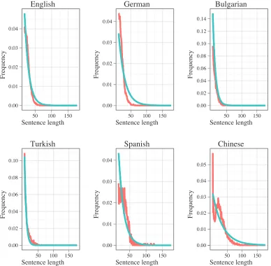
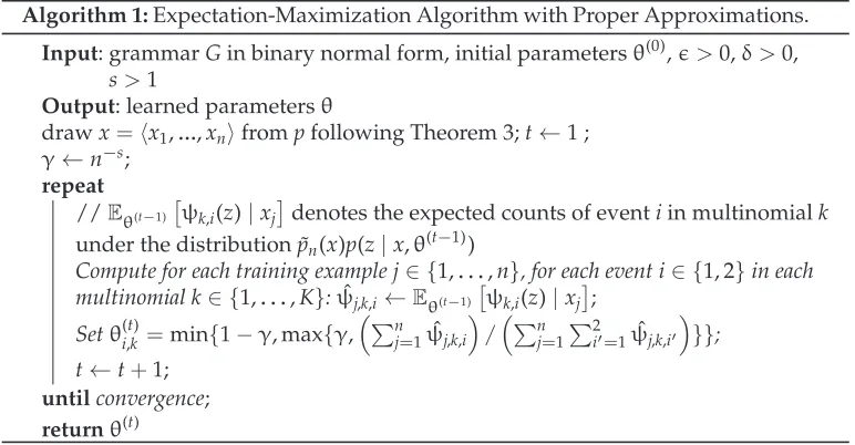
Figure 1 shows the frequency of sentence length for treebanks in various lan-guages.4 The trend in the plots clearly shows that in the extended tail of the curve, all languages have an exponential decay of probabilities as a function of sentence length. To test this, we performed a simple regression of frequencies using an exponential curve. We estimated each curve for each language using a curve of the formf(l;c,α)=clα. This estimation was done by minimizing squared error between the frequency ver-sus sentence length curve and the approximate version of this curve. The data points used for the approximation are (li,pi), wherelidenotes sentence length andpidenotes
frequency, selected from the extended tail of the distribution. Extended tail here refers to all points with length longer thanl1, wherel1is the length with the highest frequency
in the treebank. The goal of focusing on the tail is to avoid approximating the head of the curve, which is actually a monotonically increasing function. We plotted the approximate curve together with a length versus frequency curve for new syntactic data. It can be seen (Figure 1) that the approximation is rather accurate in these corpora. As a consequence of this observation, we make a few assumptions aboutGand p(x,z):
r
Derivation length proportional to sentence length: There is anα≥1 such that, for allz,|z| ≤α|yield(z)|. Further,|z| ≥ |x|. (This prohibits unary cycles.)r
Exponential decay of derivations: There is a constantr<1 and a constant L≥0 such thatp(z)≤Lr|z|. Note that the assumption here is about the frequency of length of separate derivations, and not the aggregated frequency of all sentences of a certain length (cf. the discussion above referring to Figure 1).Figure 1
A plot of the tail of frequency vs. sentence length in treebanks for English, German, Bulgarian, Turkish, Spanish, and Chinese. Red lines denote data from the treebank, blue lines denote an approximation which uses an exponential function of the formf(l;c,α)=clα(the blue line uses data which is different from the data used to estimate the curve parameters,candα). The parameters (c,α) are (0.19, 0.92) for English, (0.06, 0.94) for German, (0.26, 0.89) for Bulgarian, (0.26, 0.83) for Turkish, (0.11, 0.93) for Spanish, and (0.03, 0.97) for Chinese. Squared errors are 0.0005, 0.0003, 0.0007, 0.0003, 0.001, and 0.002 for English, German, Bulgarian, Turkish, Spanish, and Chinese, respectively.
r
Bounded expectations of rules: There is aB<∞such thatEp
ψk,i(z)≤B for allkandi.
These assumptions must hold for anypwhose support consists of a finite set. These assumptions also hold in many cases whenpitself is a probabilistic grammar. Also, we note that the last requirement of bounded expectations is optional, and it can be inferred from the rest of the requirements:B=L/(1−q)2. We make this requirement explicit for simplicity of notation later. We denote the family of distributions that satisfy all of these requirements byP(α,L,r,q,B,G).
There are other cases in the literature of language learning where additional as-sumptions are made on the learned family of models in order to obtain positive learn-ability results. For example, Clark and Thollard (2004) put a bound on the expected length of strings generated from any state of probabilistic finite state automata, which resembles the exponential decay of strings we have forpin this article.
An immediate consequence of these assumptions is that the entropy ofp is finite and bounded by a quantity that depends onL,rand q.5 Bounding entropy of labels (derivations) given inputs (sentences) is a common way to quantify the noise in a distribution. Here, both thesentential entropy (Hs(p)=−
xp(x) logp(x)) is bounded
as well as thederivationalentropy (Hd(p)=−
x,zp(x,z) logp(x,z)). This is stated in the
following result.
Proposition 1
Letp∈P(α,L,r,q,B,G) be a distribution. Then, we have
Hs(p)≤Hd(p)≤ −logL+ Llogr
(1−q)2log 1r +
(1+logL)/log1 r
e Λ
1+logL log1
r
Proof
First note that Hs(p)≤Hd(p) holds by the data processing inequality (Cover and Thomas 1991) because the sentential probability distributionp(x) is a coarser version of the derivational probability distributionp(x,z). Now, considerp(x,z). For simplicity of notation, we usep(z) instead ofp(x,z). The yield ofz,x, is a function ofz, and therefore can be omitted from the distribution. It holds that
Hd(p)=−
z
p(z) logp(z)
=−
z∈Z1
p(z) logp(z)−
z∈Z2
p(z) logp(z)
=Hd(p,Z1)+Hd(p,Z2)
whereZ1 ={z|p(z)>1/e}andZ2={z|p(z)≤1/e}. Note that the function−αlogα
reaches its maximum forα=1/e. We therefore have
Hd(p,Z1)≤ |Ze1|
We give a bound on|Z1|, the number of “high probability” derivations. Because we have p(x,z)≤Lr|z|, we can find the maximum length of a derivation that has a probability of more than 1/e(and hence, it may appear inZ1) by solving 1/e≤Lr|z|for|z|, which leads
to|z| ≤log(1/eL)/logr. Therefore, there are at most(1+logL)/log 1 r
k=1 Λ(k) derivations in |Z1|and therefore we have
|Z1| ≤
(1+logL)/log 1r
Λ
(1+logL)/log 1r
Hd(p,Z1)≤
(1+logL)/log1 r
e Λ
(1+logL)/log 1r
(12)
where we use the monotonicity ofΛ. ConsiderHd(p,Z2) (the “low probability”
deriva-tions). We have:
Hd(p,Z2)≤ −
z∈Z2
Lr|z|log
Lr|z|
≤ −logL−Llogr z∈Z2
|z|r|z|
≤ −logL−Llogr
∞
k=1
Λ(k)krk
≤ −logL−Llogr
∞
k=1
kqk (13)
=−logL+ Llogr
(1−q)2 log 1q (14)
where Equation (13) holds from the assumptions about p. Putting Equation (12) and Equation (14) together, we obtain the result.
We note that another common way to quantify the noise in a distribution is through the notion of Tsybakov noise (Tsybakov 2004; Koltchinskii 2006). We discuss this further in Section 7.1, where we show that Tsybakov noise is too permissive, and probabilistic grammars do not satisfy its conditions.
3.2 Limiting the Degree of the Grammar
When approximating a family of probabilistic grammars, it is much more convenient when the degree of the grammar is limited. In this article, we limit the degree of the grammar by making the assumption that allNk≤2. This assumption may seem, at first glance, somewhat restrictive, but we show next that for PCFGs (and as a consequence, other formalisms), this assumption does not limit the total generative capacity that we can have across all context-free grammars.
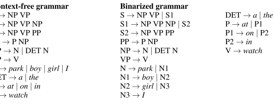
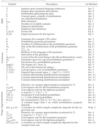
We first show that any context-free grammar with arbitrary degree can be mapped to a corresponding grammar with allNk≤2 that generates derivations equivalent to
Figure 2
Example of a context-free grammar and its equivalent binarized form.
A→αi,i<Nk, we create a new nonterminal inGsuch thatAi has two rewrite rules: Ai→αi andAi→Ai+1. In addition, we create rulesA→A1 andANk→αNk. Figure 2 demonstrates an example of this transformation on a small context-free grammar.
It is easy to verify that the resulting grammar G has an equivalent capacity to the original CFG, G. A simple transformation that converts each derivation in the new grammar to a derivation in the old grammar would involve collapsing any path of nonterminals added toG (i.e., allAi for nonterminal A) so that we end up with
nonterminals from the original grammar only. Similarly, any derivation in Gcan be converted to a derivation inGby adding new nonterminals through unary application of rules of the formAi→Ai+1. Given a derivationzinG, we denote byΥG→G(z) the
corresponding derivation inGafter adding the new non-terminalsAitoz. Throughout
this article, we will refer to the normalized form ofGas a “binary normal form.”6 Note that K, the number of multinomials in the binary normal form, is a func-tion of both the number of nonterminals in the original grammar and the number of rules in that grammar. More specifically, we have thatK=Kk=1Nk+K. To make the
equivalence complete, we need to show that anyprobabilisticcontext-free grammar can be translated to a PCFG with maxkNk≤2 such that the two PCFGs induce the same
equivalent distributions over derivations.
Utility Lemma 1
Let ai∈[0, 1], i∈ {1,. . .,N} such that
iai=1. Define b1 =a1, c1=1−a1, bi=
a
i ai−1
bi−1 ci−1
, andci=1−bifori≥2. Thenai=
i−1
j=1 cj
bi.
See AppendixA for the proof of Utility Lemma 1.
Theorem 1
LetG,θbe a probabilistic context-free grammar. LetGbe the binarizing transforma-tion ofGas defined earlier. Then, there existsθforGsuch that for any z∈D(G) we havep(z|θ,G)=p(ΥG→G(z)|θ,G).
Proof
For the grammarG, indexthe set{1,...,K}with nonterminals ranging fromA1 toAK.
DefineGas before. We need to defineθ. Indexthe multinomials inGby (k,i), each hav-ing two events. Letµ(k,i),1=θk,i,µ(k,i),2=1−θk,i fori=1 and setµk,i,1=θk,i/µ(k,i−1),2, andµ(k,i−1),2=1−µ(k,i−1),2.
G,µis a weightedcontext-free grammar such that the µ(k,i),1 corresponds to the ith event in thekmultinomial of the original grammar. Letzbe a derivation in Gand z= ΥG→G(z). Then, from Utility Lemma 1 and the construction ofg, we have that:
p(z|θ,G)=
K
k=1 Nk
i=1
θψk,ik,i(z)
=
K
k=1 Nk
i=1 ψk,i(z)
l=1
θk,i
=
K
k=1 Nk
i=1 ψk,i(z)
l=1
i−1
j=1
µ(k,j),2
µ(k,i),1
=
K
k=1 Nk
i=1
i−1
j=1
µψ(k,kj,),2i(z)
µψ(k,ki,),1i(z)
=
K
k=1 Nk
j=1 2
i=1
µψk,j(z )
(k,j),i
=p(z|µ,G)
From Chi (1999), we know that the weighted grammarG,µcan be converted to a probabilistic context-free grammar G,θ, through a construction ofθbased onµ, such thatp(z|µ,G)=p(z|θ,G).
The proof for Theorem 1 gives a construction the parametersθofGsuch thatG,θ is equivalent toG,θ. The construction ofθcan also be reversed: GivenθforG, we can constructθforGso that again we have equivalence betweenG,θandG,θ.
In this section, we focused on presenting parametrized, empirically justified distri-butional assumptions about language data that will make the analysis in later sections more manageable. We showed that these assumptions bound the amount of entropy as a function of the assumption parameters. We also made an assumption about thestructure of the grammar family, and showed that it entails no loss of generality for CFGs. Many other formalisms can follow similar arguments to show that the structural assumption is justified for them as well.
4.Proper Approximations
In order to follow the empirical risk minimization described in Section 2.1, we have to define a series of approximations forF, which we denote by the log-concept spaces
construct the sequence of concept spaces, and in Section 5 we return to the learning model. Our approximations are based on the concept ofbounded approximations(Abe, Takeuchi, and Warmuth 1991; Dasgupta 1997), which were originally designed for graphical models.7 A bounded approximation is a subset of a concept space which is controlled by a parameter that determines its tightness. Here we use this idea to define a series of subsets of the original concept spaceFas approximations, while having two asymptotic properties that control the series’ tightness.
Let Fm (for m∈ {1, 2,. . .}) be a sequence of concept spaces. We consider three
properties of elements of this sequence, which should hold form>Mfor a fixedM. The first iscontainmentinF:
Fm⊆F
The second property isboundedness:
∃Km≥0,∀f ∈Fm, E
|f| ×I{|f| ≥Km}≤bound(m)
wherebound is a non-increasing function such thatbound(m) −→
m→∞0. This states that
the expected values of functions from Fm on values larger than some Km is small.
This is required to obtain uniform convergence results in the revised empirical risk minimization model from Section 2.1. Note thatKmcan grow arbitrarily large.
The third property istightness:
∃Cm∈F→Fm, p
f∈F
{z|Cm(f)(z)−f(z)≥tail(m)}
≤tail(m)
where tail is a non-increasing function such that tail(m) −→
m→∞0, and Cm denotes an
operator that maps functions inFtoFm. This ensures that our approximation actually converges to the original concept space F. We will show in Section 4.3 that this is actually a well-motivated characterization of convergence for probabilistic grammars in the supervised setting.
We say that the sequenceFmproperly approximatesFif there existtail(m),bound(m),
andCm such that, for allmlarger than someM, containment, boundedness, and
tight-ness all hold.
In a good approximation,Km would increase at a fast rate as a function ofmand
tail(m) andbound(m) decrease quickly as a function ofm. As we will see in Section 5, we cannot have an arbitrarily fast convergence rate (by, for example, taking a subsequence ofFm), because the size ofKm has a great effect on the number of samples required to
obtain accurate estimation.
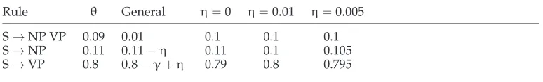
Table 1
Example of a PCFG where there is more than a single way to approximate it by truncation with γ=0.1, because it has more than two rules. Any value ofη∈[0,γ] will lead to a different approximation.
Rule θ General η=0 η=0.01 η=0.005 S→NP VP 0.09 0.01 0.1 0.1 0.1 S→NP 0.11 0.11−η 0.11 0.1 0.105 S→VP 0.8 0.8−γ+η 0.79 0.8 0.795
4.1 Constructing Proper Approximations for Probabilistic Grammars
We now focus on constructing proper approximations for probabilistic grammars whose degree is limited to 2. Proper approximations could, in principle, be used with losses other than the log-loss, though their main use is for unbounded losses. Starting from this point in the article, we focus on using such proper approximations with the log-loss.
We constructFm. For eachf ∈Fwe define a transformationT(f,γ) that shifts every
binomial parameterθk=θk,1,θk,2in the probabilistic grammar by at mostγ:
θk,1,θk,2 ←
γ, 1−γifθk,1 < γ
1−γ,γ ifθk,1 >1−γ
θk,1, θk,2 otherwise
Note thatT(f,γ)∈Ffor anyγ≤1/2. Fixa constants>1.8 We denote byT(θ,γ) the same transformation onθ(which outputs the new shifted parameters) and we denote byΘG(γ)= Θ(γ) the set{T(θ,γ)|θ∈ΘG}. For eachm∈N, define Fm ={T(f,m−s)| f ∈F}.
When considering our approach to approximate a probabilistic grammar by in-creasing its parameter probabilities to be over a certain threshold, it becomes clear why we are required to limit the grammar to have only two rules and why we are required to use the normal from Section 3.2 with grammars of degree 2. Consider the PCFG rules in Table 1. There are different ways to move probability mass to the rule with small probability. This leads to a problem with identifability of the approximation: How does one decide how to reallocate probability to the small probability rules? By binarizing the grammar in advance, we arrive at a single way to reallocate mass when required (i.e., move mass from the high-probability rule to the low-probability rule). This leads to a simpler proof for sample complexity bounds and a single bound (rather than different bounds depending on different smoothing operators). We note, however, that the choices made in binarizing the grammar imply a particular way of smoothing the probability across the original rules.
We now describe how this construction of approximations satisfies the proper-ties mentioned in Section 4, specifically, the boundedness property and the tightness property.
Proposition 2
Let p∈P(α,L,r,q,B,G) and let Fm be as defined earlier. There exists a constantβ=
β(L,q,p,N)>0 such thatFm has the boundedness property withKm =sNlog3mand
bound(m)=m−βlogm.
See AppendixA for the proof of Proposition 2.
Next,Fmis tight with respect toFwithtail(m)=
Nlog2m ms−1 .
Proposition 3
Letp∈P(α,L,r,q,B,G) and letFmas defined earlier. There exists anMsuch that for any m>Mwe have
p
f∈F
{z|Cm(f)(z)−f(z)≥tail(m)}
≤tail(m)
fortail(m)= Nlog
2 m
ms−1 andCm(f)=T(f,m
−s
).
See AppendixA for the proof of Proposition 3.
We now have proper approximations for probabilistic grammars. These approx-imations are defined as a series of probabilistic grammars, related to the family of probabilistic grammars we are interested in estimating. They consist of three prop-erties: containment (they are a subset of the family of probabilistic grammars we are interested in estimating), boundedness (their log-loss does not diverge to infinity quickly), and they are tight (there is a small probability mass at which they are not tight approximations).
4.2 Coupling Bounded Approximations with Number of Samples
At this point, the number of samplesnis decoupled from the bounded approximation (Fm) that we choose for grammar estimation. To couple between these two, we need to definemas a function of the number of samples,m(n). As mentioned earlier, there is a clear trade-off between choosing a fast rate form(n) (such asm(n)=nk for some k>1) and a slower rate (such as m(n)=logn). The faster the rate is, the tighter the family of approximations that we use forn samples. If the rate is too fast, however, thenKmgrows quickly as well. In that case, because our sample complexity bounds are
increasing functions of suchKm, the bounds will degrade.
4.3 Asymptotic Empirical Risk Minimization
It would be compelling to determine whether the empirical risk minimizer overFn is
an asymptotic empirical risk minimizer. This would mean that the risk of the empirical risk minimizer overFnconverges to the risk of the maximum likelihood estimate. As a
conclusion to this section about proper approximations, we motivate the three re-quirements that we posed on proper approximations by showing that this is indeed true. We now unify n, the number of samples, andm, the indexof the approx ima-tion of the concept space F. Let fn∗ be the minimizer of the empirical risk over F, (fn∗=argminf∈FEp˜n
f) and let gn be the minimizer of the empirical risk over Fn
(gn=argminf∈FnEp˜n
f).
LetD={z1,...,zn}be a sample fromp(z). The operator (gn=) argminf∈FnEp˜n[f] is an asymptotic empirical risk minimizer ifEEp˜n
gn
−Ep˜n[f ∗
n]
→0 asn→ ∞ (Shalev-Shwartz et al. 2009). Then, we have the following
Lemma 1
Denote byZ,nthe set
f∈F{z|Cn(f)(z)−f(z)≥}. Denote byA,nthe event “one of zi∈Dis inZ,n.” IfFnproperly approximatesF, then:
EEp˜n
gn
−Ep˜n
fn∗ (15)
≤EEp˜n
Cn(fn∗)
|A,np(A,n)+E
Ep˜n
fn∗|A,np(A,n)+tail(n)
where the expectations are taken with respect to the data setD.
See AppendixA for the proof of Lemma 1.
Proposition 4
LetD={z1,...,zn}be a sample of derivations fromG. Thengn=argminf∈FnEp˜n
fis an asymptotic empirical risk minimizer.
Proof
Letf0∈Fbe the concept that puts uniform weights overθ, namely,θk=12,12for allk.
Note that
|EEp˜n
fn∗|A,n
|p(A,n)
≤ |EEp˜n
f0
|A,n
|p(A,n)= log 2
n
n l=1
LetAj,,nforj∈ {1,. . .,n}be the event “zj∈Z,n”. ThenA,n=
jAj,,n. We have
that
E[ψk,i(zl)|A,n]p(A,n)≤
j
zl
p(zl,Aj,,n)|zl|
≤ j=l
zl
p(zl)p(Aj,,n)|zl|+
zl
p(zl,Al,,n)|zl| (16)
≤
j=l
p(Aj,,n)
B+E[ψk,i(z)|z∈Z,n]p(z∈Z,n)
≤(n−1)Bp(z∈Z,n)+E[ψk,i(z)|z∈Z,n]p(z∈Z,n)
where Equation (16) comes from zl being independent. Also, B is the constant from
Section 3.1. Therefore, we have:
1 n
n
l=1
k,i
E[ψk,i(zl)|A,n]p(A,n)
≤ k,i
E[ψk,i(z)|z∈Z,n]p(z∈Z,n)+(n−1)Bp(z∈Z,n)
From the construction of our proper approximations (Proposition 3), we know that only derivations of length log2nor greater can be inZ,n. Therefore
E[ψk,i|Z,n]p(Z,n)≤
z:|z|>log2n
p(z)ψk,i(z)≤
∞
l>log2n
LΛ(l)rll≤κqlog2n=o(1)
where κ >0 is a constant. Similarly, we have p(z∈Z,n)=o(n−1). This means that |E[Ep˜n[−log−f
∗
n]|A,n]|p(A,n) −→
n→∞0. In addition, it can be shown that|E[Ep˜n[Cn(f ∗
n)| A,n]|p(A,n) −→
n→∞0 using the same proof technique we used here, while relying on the
fact thatCn(fn∗)∈Fn, and thereforeCn(fn∗)(z)≤sN|z|logn.
5.Sample Complexity Bounds
Equipped with the framework of proper approximations as described previously, we now give our main sample complexity results for probabilistic grammars. These results hinge on the convergence of supf∈F
n|Ep˜n
f−Ep
f|. Indeed, proper approximations replace the use ofFin these convergence results. The rate of this convergence can be fast, if thecovering numbersforFndo not grow too fast.
5.1 Covering Numbers and Bounds on Covering Numbers
be a class of functions. Letd(f,g) be a distance measure between two functionsf,gfrom
G. An-cover is a subset ofG, denoted byG, such that for everyf ∈Gthere exists an f∈Gsuch thatd(f,f)< . Thecovering numberN(,G,d) is the size of the smallest -cover ofGfor the distance measured.
We are interested in a specific distance measure which is dependent on the empirical distribution ˜pnthat describes the dataz1,...,zn. Letf,g∈G. We will use
dp˜n(f,g)=E
˜ pn
|f −g|=
z∈D(G)|f(z)−g(z)|p˜n(z)
= n1
n
i=1|f(zi)−g(zi)|
Instead of using N(,G,dp˜n) directly, we bound this quantity with N(,G)=sup
˜ pn
N(,G,dp˜n), where we consider all possible samples (yielding ˜p
n). The following is the
key result regarding the connection between covering numbers and the double-sided convergence of the empirical process supf∈F
n|Ep˜n
f−Epf|asn→ ∞. This result is a general-purpose result that has been used frequently to prove the convergence of empirical processes of the type we discuss in this article.
Lemma 2
Let Fn be a permissible class9 of functions such that for everyf ∈Fnwe haveE[|f| ×
I{|f| ≤Kn}]≤bound(n). LetFtruncated,n={f×I{f ≤Kn} |f ∈Fm}, namely, the set of
functions fromFnafter being truncated byKn. Then for >0 we have
p
sup
f∈Fn
|Ep˜n
f−Ep
f|>2
≤8N(/8,Ftruncated,n) ex p
− 1 128n
2/ Kn2
+bound(n)/
providedn≥K2n/42andbound(n)< .
See Pollard (1984; Chapter 2, pages 30–31) for the proof of Lemma 2. See also Ap-pendixA.
Covering numbers are rather complexcombinatorial quantities which are hard to compute directly. Fortunately, they can be bounded using the pseudo-dimension (Anthony and Bartlett 1999), a generalization of the Vapnik-Chervonenkis (VC) dimension for real functions. In the case of our “binomialized” probabilistic grammars, the pseudo-dimension of Fn is bounded by N, because we have Fn⊆F, and the
functions in F are linear with N parameters. Hence, Ftruncated,n also has
pseudo-dimension that is at mostN. We then have the following.
Lemma 3
(From Pollard [1984] and Haussler [1992].) LetFn be the proper approximations for
probabilistic grammars, for any 0< <Knwe have:
N(,Ftruncated,n)<2
2eKn
log 2eKn
N
5.2 Supervised Case
We turn to give an analysis for the supervised case. This analysis is mostly described as a preparation for the unsupervised case. In general, the families of probabilistic grammars we give a treatment to are parametric families, and the maximum likelihood estimator for these families is a consistent estimator in the supervised case. In the unsupervised case, however, lack of identifiability prevents us from getting these traditional consis-tency results. Also, the traditional results about the consisconsis-tency of MLE are based on the assumption that the sample is generated from the parametric family we are trying to estimate. This is not the case in our analysis, where the distribution that generates the data does not have to be a probabilistic grammar.
Lemmas 2 and 3 can be combined to get the following sample complexity result.
Theorem 2
LetGbe a grammar. Letp∈P(α,L,r,q,B,G) (Section 3.1). LetFnbe a proper
approxima-tion for the corresponding family of probabilistic grammars. Letz1,. . .,zn be a sample
of derivations. Then there exists a constantβ(L,q,p,N) and constantMsuch that for any 0< δ <1 and 0< <Knand anyn>Mand if
n≥max 128K
2 n
2
2Nlog(16eKn/)+log32δ
,log 4/δ+log 1/ β(L,q,p,N)
!
then we have
P
sup
f∈Fn
|Ep˜n
f−Ep
f| ≤2
≥1−δ
whereKn=sNlog3n.
Proof Sketch
β(L,q,p,N) is the constant from Proposition 2. The main idea in the proof is to solve for nin the following two inequalities (based on Equation [17] [see the following]) while relying on Lemma 3:
8N(/8,Ftruncated,n) ex p
− 1 128n
2/K2 n
≤δ/2
bound(n)/≤δ/2
Theorem 2 gives little intuition about the number of samples required for accurate estimation of a grammar because it considers the “additive” setting: The empirical risk is withinfrom the expected risk. More specifically, it is not clear how we should pick for the log-loss, because the log-loss can obtain arbitrary values.
We turn now to converting the additive bound in Theorem 2 to a multiplicative bound. Multiplicative bounds can be more informative than additive bounds when the range of the values that the log-loss can obtain is not known a priori. It is important to note that the two views are equivalent (i.e., it is possible to convert a multiplicative bound to an additive bound and vice versa). Letρ∈(0, 1) and choose=ρKn. Then, substituting thisin Theorem 2, we get that if
n≥max 128 ρ2
2Nlog16ρe+log32 δ
,log 4/δ+log 1/ρ β(L,q,p,N)
!
then, with probability 1−δ,
sup
f∈Fn
1−
Ep˜n
f Ep
f
≤
ρ×2sNlog3(n)
H(p) (17)
whereH(p) is the Shannon entropy ofp. This stems from the fact thatEp
f≥H(p) for any f. This means that if we are interested in computing a sample complexity bound such that the ratio between the empirical risk and the expected risk (for log-loss) is close to 1 with high probability, we need to pick upρ such that the righthand side of Equation (17) is smaller than the desired accuracy level (between 0 and 1). Note that Equation (17) is an oracle inequality—it requires knowing the entropy of p or some upper bound on it.
5.3 Unsupervised Case
In the unsupervised setting, we havenyieldsof derivations from the grammar,x1,...,xn,
and our goal again is to identify grammar parametersθfrom these yields. Our concept classes are now the sets of log marginalized distributions fromFn. For eachfθ∈Fn, we
definefθ as
fθ(x)=−log
z∈Dx(G)
exp(−fθ(z))=−log
z∈Dx(G) exp
K
k=1 Nk
i=1
ψi,k(z)θi,k
We denote the set of{fθ}byFn. Analogously, we defineF. Note that we also need to define the operatorCn(f) as a first step towards definingFnas proper approximations (for F) in the unsupervised setting. Let f∈F. Let f be the concept in F such that f(x)=zf(x,z). Then we defineCn(f)(x)=zCn(f)(x,z).
It does not immediately follow that Fnis a proper approximation for F. It is not hard to show that the boundedness property is satisfied with the sameKnand the same
Utility Lemma 2
For ai,bi≥0, if −log
iai+log
ibi≥ then there exists an i such that −logai+
logbi≥.
Proposition 5
There exists anMsuch that for anyn>Mwe have
p
f∈F
{x|Cn(f)(x)−f(x)≥tail(n)}
≤tail(n)
fortail(n)=Nlog
2 n
ns−1 and the operatorCn(f) as defined earlier.
Proof Sketch
From Utility Lemma 2 we have
p
f∈F
{x|Cn(f)(x)−f(x)≥tail(n)}
≤p
f∈F
{x| ∃zCn(f)(z)−f(z)≥tail(n)}
DefineX(n) to be allxsuch that there exists azwith yield(z)=xand|z| ≥log2n. From the proof of Proposition 3 and the requirements onp, we know that there exists anα≥1 such that
p f∈F{x| ∃zs.t.Cn(f)(z)−f(z)≥tail(n)}
≤
x∈X(n) p(x)
≤
x:|x|≥log2n/α
p(x)≤
∞
k=log2n/α
LΛ(k)rk ≤tail(n)
where the last inequality happens for somenlarger than a fixedM.
Computing either the covering number or the pseudo-dimension ofFn is a hard task, because the function in the classes includes the “log-sum-exp.” Dasgupta (1997) overcomes this problem for Bayesian networks with fixed structure by giving a bound on the covering number for (his respective)Fwhich depends on the covering number ofF.
approximations of F, and the constants which control the underlying distribution p mentioned in Section 3.
Utility Lemma 3
For any two positive-valued sequences (a1,. . .,an) and (b1,. . .,bn) we have that
i|logai/bi| ≥ |log (
ai/
bi)|.
Proposition 6 (Hidden Variable Rule for Probabilistic Grammars)
Letm=
log 4Kn (1−q) log 1q
. Then,N(,Ftruncated, n)≤N
2Λ(m),Ftruncated,n
.
Proof
LetZ(m)={z| |z| ≤m}be the subset of derivations of length shorter thanm. Consider f,f0 ∈Ftruncated,n. Letfandf0be the corresponding functions inFtruncated, n. Then, for any
distributionp,
dp(f,f0)=
x
|f(x)−f0(x)|p(x)≤
x
z
|f(x,z)−f0(x,z)|p(x)
=
x
z∈Z(m)
|f(x,z)−f0(x,z)|p(x)+
x
z∈/Z(m)
|f(x,z)−f0(x,z)|p(x)
≤ x
z∈Z(m)
|f(x,z)−f0(x,z)|p(x)+
x
z∈/Z(m)
2Knp(x) (18)
≤ x
z∈Z(m)
|f(x,z)−f0(x,z)|p(x)+2Kn x:|x|≥m
|Dx(G)|p(x)
≤ x
z∈Z(m)
|f(x,z)−f0(x,z)|p(x)+2Kn
∞
k=m
Λ2(k)rk
≤dp(f,f0)|Z(m)|+2Kn qm 1−q
wherep(x,z) is a probability distribution that uniformly divides the probability mass p(x) across all derivations for the specificx, that is:
p(x,z)= p(x)
|Dx(G)|
The inequality in Equation (18) stems from Utility Lemma 3.
Setmto be the quantity that appears in the proposition to get the necessary result (fandf are arbitrary functions inFtruncated, nandFtruncated,nrespectively. Then consider f0andf0to be functions from the respective covers.).
Theorem 3
LetGbe a grammar. LetFn be a proper approximation for the corresponding family of probabilistic grammars. Letp(x,z) be a distribution over derivations which satisfies the requirements in Section 3.1. Letx1,. . .,xn be a sample of strings fromp(x). Then there
exists a constantβ(L,q,p,N) and constantMsuch that for any 0< δ <1, 0< <Kn,
anyn>M, and if
n≥max 128K
2 n
2
2Nlog
32eKnΛ(m)
+log32 δ
,log 4/δ+log 1/ β(L,q,p,N)
!
(19)
wherem=
log 4Kn (1−q) log 1q
, we have that
p
sup
f∈Fn |Ep˜n
f−Ep
f| ≤2
≥1−δ
whereKn=sNlog3n.
Theorem 3 states that the number of samples we require in order to accurately esti-mate a probabilistic grammar from unparsed strings depends on the level of ambiguity in the grammar, represented asΛ(m). We note that this dependence is polynomial, and we consider this a positive result for unsupervised learning of grammars. More specif-ically, ifΛis an exponential function (such as the case with PCFGs), when compared to the supervised learning, there is an extra multiplicative factor in the sample complexity in the unsupervised setting that behaves likeO(log logKn).
We note that the following Equation (20) can again be reduced to a multiplicative case, similarly to the way we described it for the supervised case. Setting=ρKn(ρ∈
(0, 1)), we get the following requirement onn:
n≥max 128 ρ2
2Nlog
32e×t(ρ) ρ
+log32 δ
,log 4/δ+log 1/ β(L,q,p,N)
!
(20)
wheret(ρ)=
log 4
ρ(1−q) log 1q
.
6.Algorithms for Empirical Risk Minimization
We turn now to describing algorithms and their properties for minimizing empirical risk using the framework described in Section 4.
6.1 Supervised Case