Composition for Distributional Semantics
David Weir
∗ University of SussexJulie Weeds
∗ University of SussexJeremy Reffin
∗ University of SussexThomas Kober
∗ University of SussexWe present a new framework for compositional distributional semantics in which the distribu-tional contexts of lexemes are expressed in terms of anchored packed dependency trees. We show that these structures have the potential to capture the full sentential contexts of a lexeme and provide a uniform basis for the composition of distributional knowledge in a way that captures both mutual disambiguation and generalization.
1. Introduction
This article addresses a central unresolved issue in distributional semantics: how to model semantic composition. Although there has recently been considerable interest in this problem, it remains unclear what distributional composition actually means. Our view is that distributional composition is a matter of contextualizing the lexemes being composed. This goes well beyond traditional word sense disambiguation, where each lexeme is assigned one of a fixed number of senses. Our proposal is that composition involves deriving a fine-grained characterization of the distributional meaning of each lexeme in the phrase, where the meaning that is associated with each lexeme is bespoke to that particular context.
Distributional composition is, therefore, a matter of integrating the meaning of each of the lexemes in the phrase. To achieve this we need a structure within which all of the lexemes’ semantics can be overlaid. Once this is done, the lexemes can collectively agree on the semantics of the phrase, and in so doing, determine the semantics that they have
∗Department of Informatics, University of Sussex. Falmer, Brighton BN1 9QH, UK. E-mail:{d.j.weir, j.e.weeds, j.p.reffin, t.kober}@sussex.ac.uk.
Submission received: 10 April 2015; revised version received: 17 April 2016; accepted for publication: 20 April 2016.
in the context of that phrase. Our process of composition thus creates a single structure that encodes contextualized representations of every lexeme in the phrase.
The (uncontextualized) distributional knowledge of a lexeme is typically formed by aggregating distributional features across alluses of the lexeme found within the corpus, where distributional features arise from co-occurrences found in the corpus. The distributional features of a lexeme are associated with weights that encode the strength of that feature. Contextualization involves inferring adjustments to these weights to reflect the context in which the lexeme is being used. The weights of distributional features that don’t fit the context are reduced, while the weight of those features that are compatible with the context can be boosted.
As an example, consider how we contextualize the distributional features of the wordwoodenin the context of the phrasewooden floor. The uncontextualized represen-tation ofwoodenpresumably includes distributional features associated with different uses, for example, The director fired the wooden actorand I sat on the wooden chair. So, although we may have observed in a corpus that it is plausible for the adjectivewooden
to modifyfloor,table,toy,actor, andvoice, in the specific context of the phrasewooden floor, we need to find a way to down-weight the distributional features of being something that can modifyactorandvoice, while up-weighting the distributional features of being something that can modifytableandtoy.
In this example we considered so-called first-order distributional features; these involve a single dependency relation (e.g., an adjective modifying a noun). Similar inferences can also be made with respect to distributional features that involve higher-order grammatical dependencies.1For example, suppose that we have observed that a noun thatwoodenmodifies (e.g.,actor) can be the direct object of the verbfired, as inThe director fired the wooden actor. We want this distributional feature ofwoodento be down-weighted in the distributional representation ofwoodenin the context ofwooden table, since things made of wood do not typically lose their job.
In addition to specializing the distributional representation of woodto reflect the context wooden floor, the distributional representation of floor should also be refined, down-weighting distributional features arising in contexts such asPrices fell through the floor, while up-weighting distributional features arising in contexts such asI polished the concrete floor.
In our example, some of the distributional features ofwooden—in particular, those to do with the noun that this sense ofwoodencould modify—areinternalto the phrase
wooden floor in the sense that they are alternatives to one of the words in the phrase. Although it is specifically afloorthat iswooden, our proposal is that the contextualized representation ofwoodenshould recognize that it is plausible that nouns such aschair
and toy could be modified by the particular sense of woodenthat is being used. The remaining distributional features areexternalto the phrase. For example, the verbmop
could be an external feature, because things that can be modified bywoodencan be the direct object ofmop. The external features ofwoodenandfloorwith respect to the phrase
wooden floorprovide something akin to the traditional interpretation of the distributional semantics of the phrase, namely, a representation of those (external) contexts in which this phrase can occur.
Although internal features are, in a sense, inconsistent with the specific semantics of the phrase, they provide a way to embellish the characterization of the distributional
meaning of the lexemes in the phrase. Recall that our goal is to infer a rich and fine-grained representation of the contextualized distributional meaning of each of the lexemes in the phrase.
Having introduced the proposal that distributional composition should be viewed as a matter of contextualization, the question arises as to how to realize this conception. Because each lexeme in the phrase needs to be able to contribute to the contextualization of the other lexemes in the phrase, we need to be able to align what we know about each of the lexeme’s distributional features so that this can be achieved. The problem is that the uncontextualized distributional knowledge associated with the different lexemes in the phrase take a different perspective on the feature space. To overcome this we need to: (a) provide a way of structuring the distributional feature space, which we do by typing distributional features with dependency paths; and (b) find a way to systematically modify the perspective that each lexeme has on this structured feature space in such a way that they are all aligned with one another.
Following Baroni and Lenci (2010), we use typed dependency relations as the bases for our distributional features, and following Pad ´o and Lapata (2007), we in-clude higher-order dependency relations in this space. However, in contrast to previ-ous proposals, the higher-order dependency relations provides structure to the space that is crucial to our definition of composition. Each co-occurrence associated with a lexeme such aswooden is typed by the path in the dependency tree that connects the lexeme wooden with the co-occurring lexeme (e.g., fired). This allows us to en-code a lexeme’s distributional knowledge with a hierarchical structure that we call an Anchored Packed Dependency Tree (APT). As we show, this data structure provides a way for us to align the distributional knowledge of the lexemes that are being com-posed in such a way that the inferences needed to achieve contextualization can be implemented.
2. The Distributional Lexicon
In this section, we begin the formalization of our proposal by describing the distribu-tional lexicon: a collection of entries that characterize the distribudistribu-tional semantics of lexemes. Table 1 provides a summary of the notation that we are using.
LetVbe a finite alphabet of lexemes,2where each lexeme is assumed to incorporate a part-of-speech tag; let Rbe a finite alphabet of grammatical dependency relations; and letTV,Rbe the set of dependency trees where every node is labeled with a member
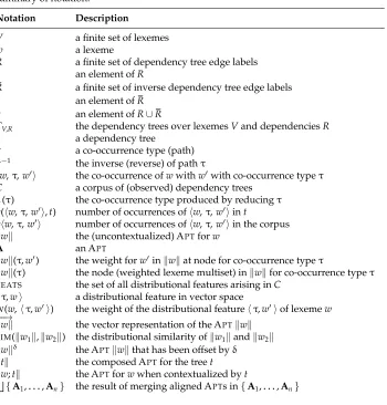
ofV, and every directed edge is labeled with an element of R. Figure 1 shows eight examples of dependency trees.
2.1 Typed Co-occurrences
When two lexemeswandw0co-occur in a dependency tree3 int∈T
V,R, we represent
this co-occurrence as a triplehw,τ,w0iwhereτis a string that encodes theco-occurrence typeof this co-occurrence, capturing the syntactic relationship that holds between these
2 There is no reason why lexemes could not include multi-word phrases tagged with an appropriate part of speech.
Table 1
Summary of notation.
Notation Description
V a finite set of lexemes
w a lexeme
R a finite set of dependency tree edge labels
r an element ofR
R a finite set of inverse dependency tree edge labels
r an element ofR
x an element ofR∪R
TV,R the dependency trees over lexemesVand dependenciesR
t a dependency tree
τ a co-occurrence type (path)
τ−1 the inverse (reverse) of pathτ
hw,τ,w0i the co-occurrence ofwwithw0with co-occurrence typeτ
C a corpus of (observed) dependency trees
↓(τ) the co-occurrence type produced by reducingτ
#(hw,τ,w0i,t) number of occurrences ofhw,τ,w0iint
#hw,τ,w0i number of occurrences ofhw,τ,w0iin the corpus
kwk the (uncontextualized) APTforw
A an APT
kwk(τ,w0) the weight forw0inkwkat node for co-occurrence typeτ
kwk(τ) the node (weighted lexeme multiset) inkwkfor co-occurrence typeτ
FEATS the set of all distributional features arising inC
hτ,wi a distributional feature in vector space
W(w,hτ,w0i) the weight of the distributional featurehτ,w0iof lexemew
−−→
kwk the vector representation of the APTkwk
SIM(kw1k,kw2k) the distributional similarity ofkw1kandkw2k
kwkδ the A
PTkwkthat has been offset byδ
ktk the composed APTfor the treet
kw;tk the APTforwwhen contextualized byt
F{
A1,. . .,An} the result of merging aligned APTs in{A1,. . .,An}
occurrences of the two lexemes. In particular,τencodes the sequence of dependencies that lie along the path intbetween the occurrences ofwandw0int. In general, a path fromwtow0intinitially travels up towards the root oft(against the directionality of the dependency edges) until an ancestor ofw0is reached. It then travels down the tree tow0(following the directionality of the dependencies). The stringτmust, therefore, not only encode the sequence of dependency relations appearing along the path, but also whether each edge is traversed in a forward or backward direction. In particular, given the pathhv0,. . .,vkiint, wherek>0,wlabelsv0, andw0labelsvk, the stringτ=x1. . .xk
encodes the co-occurrence type associated with this path as follows:
r
If the edge connectingvi−1andviruns fromvi−1toviand is labeled byr,thenxi=r.
r
If the edge connectingvi−1andviruns fromvitovi−1and is labeled byr,Hence, co-occurrence types are strings inR∗R∗, whereR={r|r∈R}.
It is useful to be able to refer to theorderof a co-occurrence type, where this simply refers to the length of the dependency path. It is also convenient to be able to refer to the inverse of a co-occurrence type. This can be thought of as the same path, but traversed in the reverse direction. To be precise, given the co-occurrence typeτ=x1·. . .·xnwhere
eachxi∈R∪Rfor 1≤i≤n, the inverse ofτ, denotedτ−1, is the pathxn−1·. . .·x1−1 wherer−1 =randr−1=rforr∈R. For example, the inverse of AMOD·DOBJ·NSUBJis
NSUBJ·DOBJ·AMOD.
The following typed co-occurrences for the lexemewhite/JJarise in the tree shown in Figure 1(a).
hwhite/JJ, AMOD·DOBJ·NSUBJ,we/PRPi hwhite/JJ, AMOD·AMOD,fizzy/JJi
hwhite/JJ, AMOD·DOBJ,bought/VBDi hwhite/JJ, AMOD·AMOD,dry/JJi
hwhite/JJ, AMOD·DET,the/DTi hwhite/JJ,,white/JJi
hwhite/JJ, AMOD·AMOD·ADVMOD,slightly/RBi hwhite/JJ, AMOD,wine/NNi
Notice that we have included the co-occurrence hwhite/JJ,,white/JJi. This gives a uniformity to our typing system that simplifies the formulation of distributional com-position in Section 4, and leads to the need for a refinement to our co-occurrence type en-codings. Because we permit paths that traverse both forwards and backwards along the same dependency—for example, in the co-occurrencehwhite/JJ,AMOD·AMOD,dry/JJi— it is logical to considerhwhite/JJ, AMOD·DOBJ·DOBJ·AMOD,dry/JJia valid co-occurrence. However, in line with our decision to include hwhite/JJ,,white/JJi rather than
hwhite/JJ, AMOD·AMOD,white/JJi, all co-occurrence types are canonicalized through a dependency cancellation process in which adjacent, complementary dependencies are cancelled out. In particular, all occurrences within the string of either rr or rr for
r∈Rare replaced with, and this process is repeated until no further reductions are possible.
The reduced co-occurrence type produced from τis denoted↓(τ), and defined as follows:
↓(τ)=
↓
(τ1τ2) ifτ=τ1r rτ2orτ=τ1r rτ2for somer∈R
τ otherwise (1)
For the remainder of this article, we only consider reduced co-occurrence types when associating a type with a co-occurrence.
Given a tree t∈TV,R, lexemes w and w0, and reduced co-occurrence type τ, the
number of times that the co-occurrencehw,τ,w0ioccurs intis denoted #(hw,τ,w0i,t), and, given some corpusCof dependency trees, the sum of all #(hw,τ,w0i,t) across all
t∈Cis denoted #hw,τ,w0i. Note that in order to simplify our notation, the dependence on the corpusCis not expressed in our notation.
we/PRPbought/VBD the/DTslightly/RB fizzy/JJdry/JJwhite/JJwine/NN NSUBJ
DOBJ DET
ADVMOD
AMOD AMOD
AMOD
(a)
your/PRP$ dry/JJ joke/NN caused/VBD laughter/NN POSS
AMOD NSUBJ DOBJ
(b)
he/PRPfolded/VBD the/DT clean/JJ dry/JJ clothes/NNS nsubj
DOBJ DET
AMOD AMOD
(c)
your/PRP$clothes/NNSlook/VBP great/JJ POSS NSUBJ XCOMP
(d)
the/DT man/PRPhung/VBD up/RP the/DTwet/JJclothes/NNS
DET NSUBJ PRT
DOBJ
DET AMOD
(e)
a/DTboy/PRPbought/VBD some/DTvery/RB expensive/JJ clothes/NNS yesterday/NN DET NSUBJ
DET
ADVMOD AMOD DOBJ
TMOD
(f)
she/PRPfolded/VBDup/RP all/DT of/IN the/DTlaundry/NNS NSUBJ PRT
DOBJ CASE
DET NMOD
(g)
he/PRPfolded/VBD under/INpressure/NN
NSUBJ CASE
NMOD
[image:6.486.48.403.61.524.2](h)
Figure 1
A small corpus of dependency trees.
we denote the weight of the distributional feature hτ,w0i of the lexemew with the expressionW(w,hτ,w0i).
2.2 Anchored Packed Trees
Given a dependency tree corpusC⊂TV,Rand a lexemew∈V, we are interested in
are central to the proposals in this article: Not only can they be used to encode the aggregate of all distributional features of a lexeme over a corpus of dependency trees, but they can also be used to express the distributional features of a lexeme that has been contextualized within some dependency tree (see Section 4).
The APTforwgivenCis denotedkwk, and referred to as theelementary APTfor
w. In the following discussion, we describe a tree-based interpretation ofkwk, but in the first instance we define it as a mapping from pairs (τ,w0) whereτ∈R∗R∗andw0∈V, such thatkwk(τ,w0) gives the weight of the typed co-occurrencehw,τ,w0iin the corpus
C. It is nothing more than those components of the weight function that specify the weights of distributional features ofw. In other words, for eachτ∈R∗R∗andw0∈V:
kwk(τ,w0)=W(w,hτ,w0i) (2)
The restriction ofkwkto co-occurrence types that are at most orderkis referred to as ak-th order APT. Thedistributional lexiconderived from a corpusCis a collection of lexical entries where the entry for the lexemewis the elementary APTkwk.
Formulating APTs as functions simplifies the definitions that appear herein. How-ever, because an APTencodes co-occurrences that are aggregated over a set of depen-dency trees, they can also be interpreted as having a tree structure. In our tree-based interpretation of APTs, nodes are associated with weighted multisets of lexemes. In particular,kwk(τ) is thought of as a node that is associated with the weighted lexeme multiset in which the weight ofw0in the multiset is kwk(τ,w0). We refer to the node
kwk() as theanchorof the APTkwk.
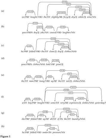
Figure 2 shows three elementary APTs that can be produced from the corpus shown in Figure 1. On the far left we give the letter corresponding to the sentence in Figure 1 that generated the typed co-occurrences. Each column corresponds to one node in the APT, giving the multiset of lexemes at that node. Weights are not shown, and only
non-empty nodes are displayed.
It is worth dwelling on the contents of the anchor node of the top APT in Figure 2, which is the elementaryAPT fordry/JJ. The weighted multiset at the anchor node is denoted kwk(). The lexeme dry/JJ occurs three times, and the weight
kwk(,dry/JJ) reflects this count. Three other lexemes also occur at this same node:
fizzy/JJ, white/JJ, and clean/JJ. These lexemes arose from the following co-occurrences in trees in Figure 1: hdry/JJ, AMOD·AMOD,fizzy/JJi, hdry/JJ, AMOD·AMOD,white/JJi, and
hdry/JJ,AMOD·AMOD,clean/JJi, all of which involve the co-occurrence type AMOD·AMOD. These lexemes appear in the multisetkwk() because↓(AMOD·AMOD)=.
3. APTSimilarity
One of the most fundamental aspects of any treatment of distributional semantics is that it supports a way of measuring distributional similarity. In this section, we describe a straightforward way in which the similarity of two APTs can be measured through a mapping from APTs to vectors.
First, define the set of distributional features
FEATS=hτ,w0iw0∈V,τ∈R∗R∗andW(w,hτ,w0i)>0 for somew∈V (3)
(a) we bought ... the slightly fizzy wine ... ... ..
. ... ... ... ... dry ... ... ... ..
. ... ... ... ... white ... ... ...
(b) ... ... your ... ... dry joke caused laughter
(c) he folded ... the ... clean clothes ... ...
..
. ... ... ... ... dry ... ... ... anchor
NSUBJ
DOBJ POSS
DET
ADVMOD AMOD NSUBJ DOBJ
(c) ... he folded ... ... the ... clean clothes ... ... ...
..
. ... ... ... ... ... ... dry ... ... ... ... (d) ... ... ... ... your ... ... ... clothes look great ...
(e) the man hung up ... the ... wet clothes ... ... ...
(f) a boy bought ... ... some very expensive clothes ... ... yesterday
anchor
DET NSUBJ PRP
POSS
DET
ADVMOD AMOD NSUBJ DOBJ
XCOMP TMOD
(c) he folded ... ... ... the clean clothes ... ... ... ..
. ... ... ... ... ... dry ... ... ... ...
(g) she folded up ... ... ... ... all of the laundry
(h) he folded ... under pressure ... ... ... ... ... ... anchor
NSUBJ PRP NMOD
CASE DOBJ
DET
AMOD
NMOD
[image:8.486.50.379.59.509.2]DET CASE
Figure 2
The distributional lexicon produced from the trees in Figure 1 with the elementary APTfor
dry/JJat the top, the elementary APTforclothes/NNSin the middle, and the elementary APTfor
folded/VBDat the bottom. Part of speech tags and weights have been omitted.
Given an APT A, we denote the vectorized representation ofAwith −→A, and the value that the vector −→A has on dimension hτ,w0i is denoted−→A
hτ,w0i
. For each
hτ,w0i ∈FEATS:
−−→ kwk
hτ,w0i
whereφ(τ,w) is a path-weighting function that is intended to reflect the fact that not all of the distributional features are equally important in determining the distributional similarity of two APTs. Generally speaking, syntactically distant co-occurrences pro-vide a weaker characterization of the semantics of a lexeme than co-occurrences that are syntactically closer. By multiplying each W(w,hτ,w0i) by φ(τ,w), we are able to capture this, given a suitable instantiation ofφ(τ,w).
One option forφ(τ,w) is to usep(τ|w)—that is, the probability that when randomly selecting one of the co-occurrenceshw,τ0,w0i, wherew0can be any lexeme inV,τ0is the co-occurrence typeτ. We can estimate these path probabilities from the co-occurrence counts inCas follows:
p(τ|w)= #hw,τ,∗i
#hw,∗,∗i (5)
where
#hw,τ,∗i= P
w0∈V#hw,τ,w0i
#hw,∗,∗i= P
w0∈VPτ∈R¯∗R∗#hw,τ,w0i
p(τ|w) typically falls off rapidly as a function of the length ofτas desired.
The similarity of two APTs, A1 and A2, which we denote SIM(A1,A2), can be measured in terms of the similarity of vectors−A→1and
−→
A2. The similarity of vectors can be measured in a variety of ways (Lin 1998; Lee 1999; Weeds and Weir 2005; Curran 2004). One popular option involves the use of the cosine measure:
SIM(A1,A2)=cos(
−→
A1,
−→
A2) (6)
It is common to apply cosine to vectors containing positive pointwise mutual informa-tion (PPMI) values. If the weights used in the APTs are counts or probabilities, then they can be transformed into PPMI values at this point.
As a consequence of the fact that the different occurrence types of the co-occurrences associated with a lexeme are being differentiated, vectorized APTs are
much sparser than traditional vector representations used to model distributional semantics. This can be mitigated in various ways, including:
r
reducing the granularity of the dependency relations and/or thepart-of-speech tag set
r
applying various normalizations of lexemes such as case normalization,lemmatization, or stemming
r
disregarding all distributional features involving co-occurrence types overa certain length
r
applying some form of distributional smoothing, where distributional4. Distributional Composition
In this section we turn to the central topic of the article, namely, distributional composi-tion. We begin with an informal explanation of our approach, and then present a more precise formalization.
4.1 Discussion of Approach
Our starting point is the observation that although we have shown that all of the elementary APTs in the distributional lexicon can be placed in the same vector space
(see Section 3), there is an important sense in which APTs for different parts of speech
are not comparable. For example, many of the dimensions that make sense for verbs, such as those involving a co-occurrence type that begins withDOBJorNSUBJ, do not make sense for a noun. However, as we now explain, the co-occurrence type structure present in an APT allows us to address this, making way for our definition of distributional composition.
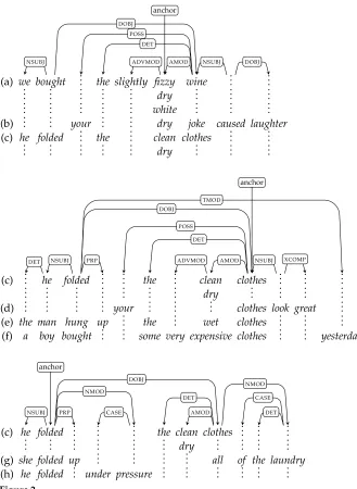
Consider the APT for the lexeme dry/JJshown at the top of Figure 2. The anchor of this APT is the node at which the lexeme dry/JJappears. We can, however, take a different perspective on this APT—for example, one in which the anchor is the node at which the lexemes bought/VBDand folded/VBDappear. This APTis shown at the top of Figure 3. Adjusting the position of the anchor is significant because the starting point of the paths given by the co-occurrence types change. For example, when the APT
shown at the top of Figure 3 is applied to the co-occurrence type NSUBJ, we reach the node at which the lexemes we/PRPand he/PRPappear. Thus, this APT can be seen as a characterization of the distributional properties of the verbs that nouns that dry/JJ modifies can take as their direct object. In fact, it looks rather like the elementary APT
for some verb. The lower tree in Figure 3 shows the elementary APT for clothes/NNS (the center APTshown in Figure 2), where the anchor has been moved to the node at which the lexemesfolded/VBD,hung/VBD, andbought/VBDappear.
Notice that in both of the APTs shown in Figure 3, parts of the tree are shown in faded text. These are nodes and edges that are removed from the APTas a result of the change in anchor placement. The elementary tree for dry/JJshown in Figure 2 reflects the fact that at least some of the nouns that dry/JJmodifies can be the direct object of a verb, or the subject of a verb. When we move the anchor, as shown at the top of Figure 3, we resolve this ambiguity to the case where the noun being modified is a direct object. The incompatible parts of the APTare removed. This corresponds to restricting the co-occurrence types of composed APTs to those that belong to the setR∗R∗, just as was the case for elementary APTs. For example, note that in the upper APT of Figure 3, neither the pathDOBJ·NSUBJfrom the node labeled with bought/VBD and folded/VBDto the node labeledcaused/VBD, nor the pathDOBJ· SUBJ· DOBJfrom the node labeled with
bought/VBDand folded/VBDto the node labeled laughter/NN, are inR∗R∗.
Given a sufficiently rich elementary APT for dry/JJ, those verbs that have nouns thatdry/JJcan plausibly modify as direct objects have elementary APTs that are in some sense “compatible” with the APTproduced by shifting the anchor node as illustrated at the top of Figure 3. An example is the APT for folded/VBDshown at the bottom of Figure 2. Loosely speaking, this means that, when applied to the same co-occurrence type, the APTin Figure 3 and the APTat the bottom of Figure 2 are generally expected to give sets of lexemes with related elements.
(a) we bought ... the slightly fizzy wine ... ...
..
. ... ... ... ... dry ... ... ...
..
. ... ... ... ... white ... ... ...
(b) ... ... your ... ... dry joke caused laughter
(c) he folded ... the ... clean clothes ... ...
..
. ... ... ... ... dry ... ... ... anchor
NSUBJ
DOBJ POSS
DET
ADVMOD AMOD NSUBJ DOBJ
(c) ... he folded ... ... the ... clean clothes ... ... ...
..
. ... ... ... ... ... ... dry ... ... ... ... (d) ... ... ... ... your ... ... ... clothes look great ...
(e) the man hung up ... the ... wet clothes ... ... ...
(f) a boy bought ... ... some very expensive clothes ... ... yesterday
anchor
DET NSUBJ PRP
POSS
DET
ADVMOD AMOD NSUBJ
DOBJ
XCOMP
[image:11.486.50.382.61.375.2]TMOD
Figure 3
The elementary APTs fordry/JJandclothes/NNSwith anchors offset.
nodes they correspond to in the APTfor folded/VBD. Not only does this make it possible, in principle at least, to establish whether or not the composition of dry/JJ, clothes/NNS, andfolded/VBDis plausible, but it provides the basis for the contextualization of APTs, as we now explain.
Recall that elementary APTs are produced by aggregating contexts taken from all of the occurrences of the lexeme in a corpus. As described in the Introduction, we need a way to contextualize aggregated APTs in order to produce a fine-grained characterization of the distributional semantics of the lexeme in context. There are two distinct aspects to the contextualization of APTs, both of which can be captured through
APTcomposition:co-occurrence filtering—the down-weighting of co-occurrences that
are not compatible with the way the lexeme is being used in its current context; and co-occurrence embellishment—the up-weighting of compatible co-occurrences that appear in the APTs for the lexemes with which it is being composed.
each of the other APTs. The second step of this process involves merging nodes that have been matched up with one another in order to produce the resulting composed APT that represents the distributional semantics of the dependency tree. It is during this second step that we are in a position to determine those co-occurrences that are compatible across the nodes that have been matched up.
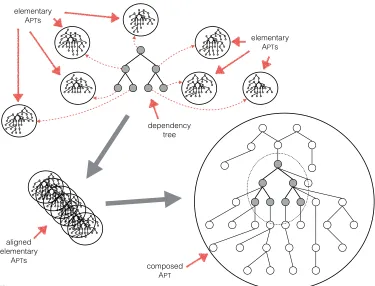
Figure 4 illustrates the composition of APTs on the basis of a dependency tree shown in the upper center of the figure. In the lower right, the figure shows the full APT that results from merging the six aligned APTs, one for each of the lexemes in the dependency tree. Each node in the dependency tree is labeled with a lexeme, and around the dependency tree we show the elementary APTs for each lexeme. The
six elementary APTs are aligned on the basis of the position of their lexeme in the dependency tree. Note that the tree shown in gray within the APT is structurally identical to the dependency tree in the upper center of the figure. The nodes of the dependency tree are labeled with single lexemes, whereas each node of the APT is labeled by a weighted lexeme multiset. The lexeme labeling a node in the dependency tree is one of the lexemes found in the weighted lexeme multiset associated with the corresponding node within the APT. We refer to the nodes in the composed APTthat come from nodes in the dependency tree (the gray nodes) as theinternal context, and the remaining nodes as theexternal context.
As we have seen, the alignment of APTs can be achieved by adjusting the location of the anchor. The specific adjustments to the anchor locations are determined by the dependency tree for the phrase. For example, Figure 5 shows a dependency analysis of
dependency tree
composed APT aligned
elementary APTs
elementary APTs
[image:12.486.52.427.355.641.2]elementary APTs
Figure 4
folded/VBD dry/JJ clothes/NNS DOBJ
AMOD
Figure 5
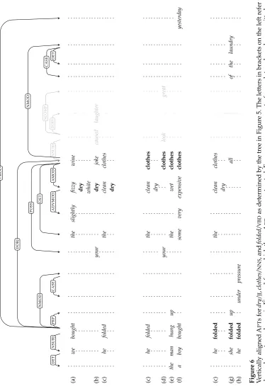
A dependency tree that generates the alignment shown in Figure 6.
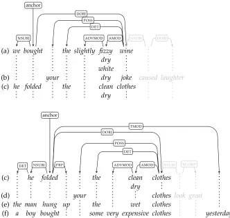
the phrasefolded dry clothes. To align the elementary APTs for the lexemes in this tree,
we do the following:
r
The anchor of the elementary APTfordry/JJis moved to the node on which thebought/VBDandfolded/VBDlie. This is the APTshown at the top of Figure 6. This change of anchor location is determined by the path from thedry/JJtofolded/VBDin the tree in Figure 5 (i.e., AMOD·DOBJ).r
The anchor of the elementary APTforclothes/NNSis moved to the node on which folded/VBD, hung/VBD, and bought/VBDlie. This is the APTshown at the bottom of Figure 3. This change of anchor location is determined by the path from the clothes/NNSto folded/VBDin the tree in Figure 5 (i.e., DOBJ).r
The anchor of the elementary APTfor folded/VBDhas been left unchanged because there is an empty path from folded/VBDto folded/VBDin the tree in Figure 5.Figure 6 shows the three elementary APTs for the lexemes dry/JJ, clothes/NNS, and
folded/VPD, which have been aligned as determined by the dependency tree shown in Figure 5. Each column of lexemes appears at nodes that have been aligned with one another. For example, in the third column from the left, we see that the following three nodes have been aligned: (i) the node in the elementary APT for dry/JJat which
bought/VBDand folded/VBDappear; (ii) the node in the elementary APT for clothes/NNS at which folded/VBD, hung/VBD, and bought/VBD appear; and (iii) the anchor node of the elementary APT for folded/VBD, that is, the node at which folded/VBD appears. In the second phase of composition, these three nodes are merged together to produce a single node in the composed APT.
Before we discuss how the nodes in aligned APTs are merged, we formalize the notion of APT alignment. We do this by first defining so-called offset APTs, which formalizes the idea of adjusting the location of an anchor. We then define how to align all of the APTs for the lexemes in a phrase based on a dependency tree.
4.2 Offset APTs
As shown in Equation (7), path offset can be specified by making use of the co-occurrence type reduction operator that was introduced in Section 2.2. Given a string
δinR∗R∗and an APT A, the offset APT Aδ is defined as follows. For each τ∈R∗R∗
andw∈V:
Aδ(τ,w)=A(↓(δτ),w) (7)
or equivalently, for eachτ∈R∗R∗:
Aδ(τ)=A(↓(δτ)) (8)
As required, Equation (7) defines Aδ by specifying the weighted lexeme multiset we obtain whenAδ is applied to co-occurrence typeτ as being the lexeme multiset thatAproduces when applied to the co-occurrence type↓(δτ).
As an illustrative example, consider the APT shown at the top of Figure 2. Let us call this APTA. Note thatAis anchored at the node where the lexeme dry/JJappears. Consider the APT produced when we apply the offset AMOD·DOBJ. This is shown at the top of Figure 3. Let us refer to this APT as A0. The anchor of A0 is the node at which the lexemes bought/VDBand folded/VBD appear. Now we show how the two nodesA0(NSUBJ) andA0(DOBJ·AMOD·ADVMOD) are defined in terms ofAon the basis of Equation (8). In both cases the offsetδ= AMOD·DOBJ.
r
For the case whereτ=NSUBJwe haveA0(NSUBJ)=A(↓(AMOD·DOBJ·NSUBJ)) =A(AMOD·DOBJ·NSUBJ)
With respect to the anchor ofA, this correctly addresses the node at which the lexemeswe/PRPandhe/PRPappear.
r
Whereτ=DOBJ·AMOD·ADVMODwe haveA0(DOBJ·AMOD·ADVMOD)=A(↓(AMOD·DOBJ·DOBJ·AMOD·ADVMOD)) =A(↓(AMOD·AMOD·ADVMOD))
=A(↓(ADVMOD)) =A(ADVMOD)
With respect to the anchor ofA, this correctly addresses the node at which the lexemeslightly/RBappears.
In practice, the offset APT Aδ can be obtained by prepending the inverse of the path offset, δ−1, to all of the co-occurrence types in Aand then repeatedly applying the reduction operator until no further reductions are possible. In other words, if τ
4.3 Syntax-Driven APTAlignment
We now make use of offset APTs, as defined in Equation (7), as a way to align all of the APTs associated with a dependency tree. Consider the following scenario:
r
w1. . .wnis a the phrase (or sentence) where eachwi∈Vfor 1≤i≤nr
t∈TV,Ris a dependency analysis of the stringw1. . .wnr
whis the lexeme at the root oft. In other words,his the position (index) inthe phrase at which the head appears
r
kwikis the elementary APTforwifor eachi, 1≤i≤nr
δi, the offset ofwiintwith respect to the root, is the path intfromwitowh.In other words,hwi,δi,whiis a co-occurrence intfor eachi, 1≤i≤n
(Note thatδh=)
We define the distributional semantics for the treet, denotedktk, as follows:
ktk=G kw1kδ1,. . .,kwnkδn (9)
The definition of F
is considered in Section 4.4. In general, F
operates on a set of
n aligned APTs, merging them into a single APT. The multiset at each node in the resulting APT is formed by merging n multisets, one from each of the elements of
kw1kδ1,. . .,kwnkδn . It is this multiset merging operation that we focus on in Sec-tion 4.4.
Although ktk can be taken to be the distributional semantics of the tree as a whole, the same APT, when associated with different anchors (i.e., when offset in some appropriate way) provides a representation of each of the contextualized lexemes that appear in the tree.
For each i, for 1≤i≤n, the APT for wi when contextualized by its role in the
dependency treet, denotedkwi;tk, is the APTthat satisfies the equality:
kwi;tkδi =ktk (10)
Alternatively, this can also be expressed with the equality:
kwi;tk=ktkδi −1
(11)
Note thatkwh;tkandktkare identical. In other words, we take the representation of the
distributional semantics of a dependency tree to be the APTfor the lexeme at the root
of that tree that has been contextualized by the other lexemes appearing below it in the tree.
possible to compose APTs in this fully incremental way, whatever the structure in the dependency tree. The tree structure, however, is critical in determining how the adjacent APTs need to be aligned.
4.4 Merging Aligned APTs
We now turn to the question of how to implement the function F
that appears in Equation (9).F
takes a set ofn aligned APTs, {A1,. . .An}, one for each node in the
dependency treet. It merges the APTs together node by node to produce a single APT,
F
{A1,. . .An}, that represents the semantics of the dependency tree. Our discussion,
therefore, addresses the question of how to merge the multisets that appear at nodes that are aligned with each other and form the nodes of the APTbeing produced.
The elementary APT for a lexeme expresses those co-occurrences that are dis-tributionally compatible with the lexeme given the corpus. When lexemes in some phrase are composed, our objective is to capture the extent to which the co-occurrences arising in the elementary APTs are mutually compatible with the phrase as a whole. Once the elementary APTs that are being composed have been aligned, we are in a position to determine the extent to which co-occurrences are mutually compatible: Co-occurrences that need to be compatible with one another are brought together through the alignment. We consider two alternative ways in which this can be achieved.
We begin withF
INT, which provides a tight implementation of the mutual compat-ibility of co-occurrences. In particular, a co-occurrence is only deemed to be compatible with the composed lexemes to the extent that is distributionally compatible with the lexeme that it is least compatible with. This corresponds to the multiset version of intersection. In particular, for allτ∈R∗R∗andw0∈V:
G
INT
{A1,. . .,An}(τ,w0)= min
1≤i≤nAi(τ,w
0) (12)
It is clear that the effectiveness of F
INT increases as the size of C grows, and that it would particularly benefit from distributional smoothing (Dagan, Pereira, and Lee 1994), which can be used to improve plausible co-occurrence coverage by inferring co-occurrences in the APT for a lexemewbased on the co-occurrences in the APTs of distributionally similar lexemes.
An alternative to F
INT is
F
UNI, where we determine distributional compatibility of a occurrence by aggregating across the distributional compatibility of the co-occurrence for each of the lexemes being composed. In particular, for allτ∈(R∪R)∗ andw0∈V:
G
UNI
{A1,. . .,An}(τ,w0)=
X
1≤i≤n
Ai(τ,w0) (13)
Although this clearly achieves co-occurrence embellishment, whether co-occurrence filtering is achieved depends on the weighting scheme being used. For example, if negative weights are allowed, then co-occurrence filtering can be achieved.
the only lexeme appearing at an internal node is the lexeme that appears at the corre-sponding node in the dependency tree. However, this is absolutely not the objective: At each node in the internal context, we expect to find a set of alternative lexemes that are, to varying degrees, distributionally compatible with that position in the APT. We expect that a lexeme that is distributionally compatible with a substantial number of the lexemes being composed will result in a distributional feature with non-zero weight in the vectorized APT. There is, therefore, no distinction being made between internal and external nodes. This enriches the distributional representation of the contextualized lexemes, and overcomes the potential problem arising from the fact that as larger and larger units are composed, there is less and less external context around to characterize distributional meaning.
5. Experiments
In this section we consider some empirical evidence in support of APTs. First, we consider some of the different ways in which APTs can be instantiated. Second, we present a number of case studies showing the disambiguating effect of APTcomposition in adjective–noun composition. Finally, we evaluate the model using the phrase-based compositionality benchmarks of Mitchell and Lapata (2008, 2010).
5.1 Instantiating APTs
We have constructed APTlexicons from three different corpora.
r
clean wikiis a corpus used for the case studies in Section 5.2. This corpus is a cleaned 2013 Wikipedia dump (Wilson 2015) that we have tokenized, part-of-speech-tagged, lemmatized, and dependency-parsed using the Malt Parser (Nivre 2004). This corpus contains approximately 0.6 billion tokens.r
BNCis the British National Corpus. It has been tokenized, POS-tagged,lemmatized, and dependency-parsed as described in Grefenstette et al. (2013) and contains approximately 0.1 billion tokens.
r
concatis a concatenation of the ukWaC corpus (Ferraresi et al. 2008), a mid-2009 dump of the English Wikipedia and the British National Corpus. This corpus has been tokenized, POS-tagged, lemmatized, anddependency-parsed as described in Grefenstette et al. (2013) and contains about 2.8 billion tokens.
Having constructed lexicons, there are a number of hyperparameters to be explored during composition. First there is the composition operation itself. We have explored variants that take a union of the features such as addand maxand variants that take an intersection of the features such as mult, min, and intersective add, where
intersective add(a,b)=a+biffa>0 andb>0; 0 otherwise.
In the instantiation that we refer to as ascompose first, APTweights are probabilities. These are composed and transformed to PPMI scores before computing cosine similar-ities. In the instantiation that we refer to ascompose second, APT weights are PPMI scores.
There are a number of modifications that can be made to the standard PPMI calcu-lation. First, it is common (Levy, Goldberg, and Dagan 2015) to delete rare words when building co-occurrence vectors. Low-frequency features contribute little to similarity calculations because they co-occur with very few of the targets. Their inclusion will tend to reduce similarity scores across the board, but have little effect on ranking. Filtering, on the other hand, improves efficiency. In other experiments, we have found that a feature frequency threshold of 1,000 works well. On a corpus the size of Wikipedia (1.5 billion tokens), this leads to a feature space for nouns of approximately 80,000 dimensions (when including only first-order paths) and approximately 230,000 dimensions (when including paths up to order 2).
Levy, Goldberg, and Dagan (2015) also showed that the use of context distribution smoothing (cds),α=0.75, can lead to performance comparable with state-of-the-art word embeddings on word similarity tasks.
PMIα w0,w;τ
=log#hw,τ,w
0i#h∗,τ,∗iα
#hw,τ,∗i#h∗,τ,w0iα
Levy, Goldberg, and Dagan (2015) further showed that using shifted PMI, which is analogous to the use of negative sampling in word embeddings, can be advanta-geous. When shifting PMI, all values are shifted down by logkbefore the threshold is applied.
SPPMI w0,w;τ
=max (PMI w0,w;τ
−logk, 0)
Finally, there are many possible options for the path weighting function φ(τ,w). These include the path probability p(τ|w) as discussed in Section 3, constant path weighting, and inverse path length or harmonic function (which is equivalent to the dynamic context window used in many neural implementations such as GloVe [Pennington, Socher, and Manning 2014]).
5.2 Disambiguation
Here we consider the differences between using aligned and unaligned APT rep-resentations as well as the differences between using F
UNI and
F
INT when carry-ing out adjective–noun (AN) composition. From theclean wiki corpus described in Section 5.1, a small number of high-frequency nouns were chosen that are ambigu-ous or broad in meaning together with potentially disambiguating adjectives. We use thecompose first option where composition is carried out on APTs containing probabilities.
W(w,hτ,w0i)= #hw,τ,w
0i
#hw,∗,∗i
Goldberg, and Dagan (2015), wherecdsis applied withα=0.75. However, no shift is applied to the PPMI values because we have found shifting to have little or negative effect when working with relatively small corpora. Similarity is then computed using the standard cosine measure. For illustrative purposes the top ten neighbors of each word or phrase are shown, concentrating on ranks rather than absolute similarity scores.
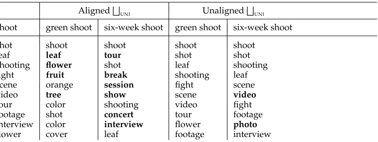
Table 2 illustrates what happens whenF
UNIis used to merge aligned and unaligned APTrepresentations when the nounshootis placed in the contexts ofgreenandsix-week. Boldface is used in the entries of compounds where a neighbor appears to be highly suggestive of the intended sense and where it has a rank higher or equal to its rank in the entry for the uncontextualized noun. In this example, it is clear that merging the unaligned APTrepresentations provides very little disambiguation of the target noun. This is because typed co-occurrences for an adjective mostly belong in a different space to typed co-occurrences for a noun. Addition of these spaces leads to significantly lower absolute similarity scores, but little change in the ranking of neighbors. Although we only show one example here, this observation appears to hold true whenever words with different part of speech tags are composed. Intersection of these spaces viaF
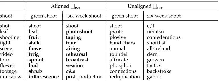
INT generally leads to substantially degraded neighbors, often little better than random, as illustrated by Table 3.
On the other hand, when APTs are correctly aligned and merged usingF
UNI, we see the disambiguating effect of the adjective. Agreen shootis more similar toleaf,flower,
fruit, and tree. Asix-week shoot is more similar to tour, session,show, and concert. This disambiguating effect is even more apparent when F
INT is used to merge the APT representations (see Table 3).
Table 4 further illustrates the difference between usingF
UNIand
F
INTwhen compos-ing aligned APTrepresentations. Again, boldface is used in the entries of compounds where a neighbor appears to be highly suggestive of the intended sense and where it has a rank higher or equal to its rank in the entry for the uncontextualized noun. In these examples, we can see that bothF
UNIand
F
INTappear to be effective in carrying out some disambiguation. Looking at the example ofmusical group, bothF
UNI and
F
INT increase the relative similarity ofbandandmusictogroupwhen it is contextualized bymusical. However,F
[image:20.486.54.433.516.659.2]INTalso leads to a number of other words being selected as neighbors that
Table 2
Neighbors of uncontextualized shoot/N compared with shoot/N in the contexts of green/J and
six-week/J, usingF
UNIwith aligned and unaligned representations.
AlignedF
UNI Unaligned
F UNI
shoot green shoot six-week shoot green shoot six-week shoot
shot shoot shoot shoot shoot
leaf leaf tour shot shot
shooting flower shot leaf shooting
fight fruit break shooting leaf
scene orange session fight scene
video tree show scene video
tour color shooting video fight
footage shot concert tour footage
interview color interview flower photo
Table 3
Neighbors of uncontextualized shoot/N compared with shoot/N in the contexts of green/J and
six-week/J, usingF
INTwith aligned and unaligned representations.
AlignedF
INT Unaligned
F INT
shoot green shoot six-week shoot green shoot six-week shoot
shot shoot shoot shoot e/f
leaf leaf photoshoot pyrite uemtsu
shooting fruit taping plosive confederations
fight stalk tour handlebars shortlist
scene flower airing annual all-ireland
video twig rehearsal roundel dern
tour sprout broadcast affricate gerwen
flower bud session phosphor tactics
footage shrub q&a connections backstroke
interview inflorescence post-production reduplication gabler
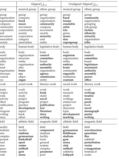
are closely related to the musical sense of group (e.g.,troupe,ensemble, andtrio). This is not the case whenF
UNI is used—the other neighbors still appear related to the general meaning ofgroup. This trend is also seen in some of the other examples such asethnic group,human body, andmagnetic field. Further, even when F
UNI leads to the successful selection of a large number of sense specific neighbors (e.g., see literary work), the neighbors selected appear to be higher frequency, more general words than whenF
INT is used.
The reason for this is likely to be the effect that each of these composition operations has on the number of non-zero dimensions in the composed representations. Ignoring the relatively small effect the feature association function may have on this, it is obvious thatF
UNI should increase the number of non-zero dimensions, whereas
F
INT should decrease the number of non-zero dimensions. In general, the number of non-zero di-mensions is highly correlated with frequency, which makes composed representations based onF
UNIbehave like high-frequency words and composed representations based on F
INT behave like low-frequency words. Further, when using similarity measures based on PPMI, as demonstrated by Weeds (2003), it is not unusual to find that the neighbors of high-frequency entities (with a large number of non-zero dimensions) are other high-frequency entities (also with a large number of non-zero dimensions). Nor is it unusual to find that the neighbors of low-frequency entities (with a small number of zero dimensions) are other low-frequency entities (with a small number of non-zero dimensions). Weeds, Weir, and McCarthy (2004) showed that frequency is also a surprisingly good indicator of the generality of the word. HenceF
UNI leads to more general neighbors andF
INTleads to more specific neighbors. Finally, note that whereas F
INT has produced high quality neighbors in these ex-amples where only two words are composed, usingF
INT in the context of the com-position of an entire sentence would tend to lead to very sparse representations. The majority of the internal nodes of the APT composed using an intersective operation such asF
INTmust necessarily only include the lexemes actually used in the sentence.
F
Table 4
Distributional neighbors usingF
UNIvs F
INT(e-magnetism = electro-magnetism).
AlignedF
UNI Unaligned Aligned
F INT
group musical group ethnic group musical group ethnic group
group group group group group
organization company organization band community
organisation band organisation troupe organization
company music community ensemble grouping
community movement company artist sub-group
corporation community movement trio faction
unit society society genre ethnicity
movement corporation minority music minority
association category unit duo organisation
society association entity supergroup tribe
body human body legislative body human body legislative body
body body body body body
board organization council organism council
organization structure committee organization committee
entity entity board entity board
skin organisation authority embryo legislature
head skin assembly brain secretariat
organisation brain organisation community authority
structure eye agency organelle assembly
council object commission institution power
eye organ entity cranium office
work social work literary work social work literary work
study work work work work
project activity book research writings
book study study study treatise
activity project novel writings essay
effort program project endeavour poem
publication practice publication project book
job development text discourse novel
program aspect literature topic monograph
writing book story development poetry
piece effort writing teaching writing
field athletic field magnetic field athletic field magnetic field
facility field field field field
stadium facility component gymnasium wavefunction
area stadium stadium fieldhouse spacetime
complex gymnasium facility stadium flux
ground basketball track gym subfield
pool sport ground arena perturbation
base center system rink vector
space softball complex softball e-magnetism
centre gym parameter cafeteria formula 8
that those internal (and external) contexts that are not supported by a majority of the lexemes in the sentence will tend to be considered insignificant and therefore will be ignored in similarity calculations. By using shifted PPMI, it should be possible to further reduce the number of non-zero dimensions in a representation constructed usingF
UNI, and this should also allow us to control the specificity/generality of the neighbors observed.
5.3 Phrase-Based Composition Tasks
Here we look at the performance of one instantiation of the APT framework on two
benchmark tasks for phrase-based composition.
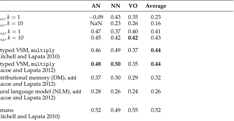
5.3.1 Experiment 1: The M&L2010 Data Set. The first experiment uses the M&L2010 data set, introduced by Mitchell and Lapata (2010), which contains human similarity judgments for adjective–noun (AN), noun–noun (NN), and verb–object (VO) combina-tions on a seven-point rating scale. It contains 108 combinacombina-tions in each category such ashsocial activity,economic conditioni,htv set,bedroom windowi, andhfight war,win battlei. This data set has been used in a number of evaluations of compositional meth-ods including Mitchell and Lapata (2010), Blacoe and Lapata (2012), Turney (2012), Hermann and Blunsom (2013), and Kiela and Clark (2014). For example, Blacoe and Lapata (2012) show that multiplication in a simple distributional space (referred to here as anuntyped VSM) outperforms the distributional memory (DM) method of Baroni and Lenci (2010) and the neural language model (NLM) method of Collobert and Weston (2008).
Although often not explicit, the experimental procedure in most of this work would appear to be the calculation of Spearman’s rank correlation coefficientρbetween model scores and individual, non-aggregated, human ratings. For example, if there are 108 phrase pairs being judged by 6 humans, this would lead to a data set containing 648 data points. The procedure is discussed at length in Turney (2012), who argues that this method tends to underestimate model performance. Accordingly, Turney explicitly uses a different procedure where a separate Spearman’sρis calculated between the model scores and the scores of each participant. These coefficients are then averaged to give the performance indicator for each model. Here, we report results using the original
M&Lmethod (see Table 5). We found that using the Turney method, scores were typically higher by 0.01 to 0.04. If model scores are evaluated against aggregated human scores, then the values of Spearman’sρtend to be still higher, typically 0.1 to 0.12 higher than the values reported here.
For this experiment, we have constructed an order 2 APTlexicon for theBNCcorpus. This is the same corpus used by Mitchell and Lapata (2010) and for the best performing algorithms in Blacoe and Lapata (2012). We note that the larger concat corpus was used by Blacoe and Lapata (2012) in the evaluation of the DM algorithm (Baroni and Lenci 2010). We use thecompose secondoption, where the elementary APTweights are PPMI. With regard to the different parameter settings in the PPMI calculation (Levy, Goldberg, and Dagan 2015), we tuned on a number of popular word similarity tasks: MEN (Bruni, Tran, and Baroni 2014); WordSim-353 (Finkelstein et al. 2001); and SimLex-999 (Hill, Reichart, and Korhonen 2015). In these tuning experiments, we found that context distribution smoothing gave mixed results. However, shifting PPMI (k=10) gave optimal results across all of the word similarity tasks. Therefore we report results here for vanilla PPMI (shift k=1) and shifted PPMI (shiftk=10). For composition, we report results for bothF
UNIand
F
Table 5
Results on the M&L2010 data set using theM&Lmethod of evaluation. Values shown are
Spearman’sρ.
AN NN VO Average
F
INT,k=1 −0.09 0.43 0.35 0.23
F
INT,k=10 NaN 0.23 0.26 0.16
F
UNI,k=1 0.47 0.37 0.40 0.41
F
UNI,k=10 0.45 0.42 0.42 0.43
untyped VSM,multiply 0.46 0.49 0.37 0.44
(Mitchell and Lapata 2010)
untyped VSM,multiply 0.48 0.50 0.35 0.44
(Blacoe and Lapata 2012)
distributional memory (DM),add 0.37 0.30 0.29 0.32
(Blacoe and Lapata 2012)
neural language model (NLM),add 0.28 0.26 0.24 0.26
(Blacoe and Lapata 2012)
humans 0.52 0.49 0.55 0.52
(Mitchell and Lapata 2010)
For this task and with this corpus, F
UNI consistently outperforms
F
INT. Shifting PPMI by log 10 consistently improves results for F
UNI, but has a large negative effect on the results for F
INT. We believe that this is due to the relatively small size of the corpus. Shifting PPMI reduces the number of non-zero dimensions in each vector, which increases the likelihood of a zero intersection. In the case of AN composition, all of the intersections were zero for this setting, making it impossible to compute a correlation.
Comparing these results with the state of the art, we can see that F
UNI clearly outperforms DM and NLM as tested by Blacoe and Lapata (2012). This method of com-position also achieves close to the best results in Mitchell and Lapata (2010) and Blacoe and Lapata (2012). It is interesting to note that our model does substantially better than the state of the art on verb–object composition, but is considerably worse at noun– noun composition. Exploring why this is so is a matter for future research. We have undertaken experiments with a larger corpus and a larger range of hyper-parameter settings, which indicate that the performance of the APTmodels can be increased signif-icantly. However, these results are not presented here, because an equitable comparison with existing models would require a similar exploration of the hyper-parameter space across all models being compared.
5.3.2 Experiment 2: The M&L2008 Data Set.The second experiment uses the M&L2008 data set, introduced by Mitchell and Lapata (2008), which contains pairs of intransitive sensitives together with human judgments of similarity. The data set contains 120 unique subject, verb, landmark triples with a varying number of human judgments per item. On average each triple is rated by 30 participants. The task is to rate the similarity of the verb and the landmark given the potentially disambiguating context of the subject. For example, in the context of the subjectfireone might expectglowedto be close toburnedbut not close tobeamed. Conversely, in the context of the subjectface
This data set was used in the evaluations carried out by Grefenstette et al. (2013) and Dinu, Pham, and Baroni (2013). These evaluations clearly follow the experimental procedure of Mitchell and Lapata and do not evaluate against mean scores. Instead, separate points are created for each human annotator, as discussed in Section 5.3.1.
The multi-step regression algorithm of Grefenstette et al. (2013) achievedρ=0.23 on this data set. In the evaluation of Dinu, Pham, and Baroni (2013), the lexical function algorithm, which learns a matrix representation for each functor and defines composi-tion as matrix-vector multiplicacomposi-tion, was the best-performing composicomposi-tional algorithm at this task. With optimal parameter settings, it achieved aroundρ=0.26. In this eval-uation, the full additive model of Guevara (2010) achievedρ <0.05.
In order to make our results directly comparable with these previous evaluations, we used the same corpus to construct our APT lexicons, namely, the concatcorpus described in Section 5.1. Otherwise, the APT lexicon was constructed as described in Section 5.3.1. As before, note thatk=1 in shifted PPMI is equivalent to not shifting PPMI. Results are shown in Table 6.
We see thatF
UNI is highly competitive with the optimized lexical function model that was the best performing model in the evaluation of Dinu, Pham, and Baroni (2013). In that evaluation, the lexical function model achieved between 0.23 and 0.26, depending on the parameters used in dimensionality reduction. Using vanilla PPMI, without any context distribution smoothing or shifting,F
UNI achievesρ=0.20, which is less than F
INT. However, when using shifted PPMI as weights, the best result is 0.26. The shifting of PPMI means that contexts need to be more surprising in order to be considered as features. This makes sense when using an additive model such as
F
UNI.
We also see that at this task and using this corpus, F
[image:25.486.54.440.481.673.2] [image:25.486.56.246.483.658.2]INT performs relatively well. Using vanilla PPMI, without any context distribution smoothing or shifting, it achievesρ=0.23, which equals the performance of the multi-step regression algorithm of Grefenstette et al. (2013). Here, however, shifting PPMI has a negative impact on performance. This is largely because of the intersective nature of the composition
Table 6
Results on the M&L2008 data set. Values shown are Spearman’sρ.
F
INT,k=1 0.23
F
INT,k=10 0.13
F
UNI,k=1 0.20
F
UNI,k=10 0.26
multi-step regression 0.23
Grefenstette et al. (2013)
lexical function 0.23–0.26
Dinu, Pham, and Baroni (2013)
untyped VSM,mult 0.20–0.22
Dinu, Pham, and Baroni (2013)
full additive 0–0.05
Dinu, Pham, and Baroni (2013)
humans 0.40
operation—if shifting PPMI removes a feature from one of the unigram representations, it cannot be recovered during composition.
6. Related Work
Our work brings together two strands usually treated as separate though related prob-lems: representing phrasal meaning by creating distributional representations through composition; and representing word meaning in context by modifying the distributional representation of a word. In common with some other work on lexical distributional similarity, we use a typed co-occurrence space. However, we propose the use of higher-order grammatical dependency relations to enable the representation of phrasal mean-ing and the representation of word meanmean-ing in context.
6.1 Representing Phrasal Meaning
The problem of representing phrasal meaning has traditionally been tackled by tak-ing vector representations for words (Turney and Pantel 2010) and combintak-ing them using some function to produce a data structure that represents the phrase or sen-tence. Mitchell and Lapata (2008, 2010) found that simple additive and multiplicative functions applied to proximity-based vector representations were no less effective than more complex functions when performance was assessed against human similarity judgments of simple paired phrases.
The word embeddings learned by the continuous bag-of-words model (CBOW) and the continuous skip-gram model proposed by Mikolov et al. (2013a, 2013b) are currently among the most popular forms of distributional word representations. Although using a neural network architecture, the intuitions behind such distributed representations of words are the same as in traditional distributional representations. As argued by Pennington et al. (2014), both count-based and prediction-based models probe the underlying corpus co-occurrences statistics. For example, the CBOW architecture pre-dicts the current word based on context (which is viewed as a bag-of-words) and the skip-gram architecture predicts surrounding words given the current word. Mikolov et al. (2013c) showed that it is possible to use these models to efficiently learn low-dimensional representations for words that appear to capture both syntactic and seman-tic regularities. Mikolov et al. (2013b) also demonstrated the possibility of composing skip-gram representations using addition. For example, they found that adding the vectors forRussianandriverresults in a very similar vector to the result of adding the vectors for Volgaandriver. This is similar to the multiplicative model of Mitchell and Lapata (2008) since the sum of two skip-gram word vectors is related to the product of two word context distributions.
Although our model shares with these the use of vector addition as a composition operation, the underlying framework is very different. Specifically, the actual vectors added depend not just on the form of the words but also their grammatical relationship within the phrase or sentence. This means that the representation for, say,glass window
is not equal to the representation ofwindow glass. The direction of the NNrelationship between the words leads to a different alignment of the APTs and consequently a different representation for the phrases.
and Guevara (2010) borrowed from formal semantics the notion that an adjective acts as a modifying function on the noun. They represented a noun as a vector, an adjective as a matrix, which could be induced from pairs of nouns and adjective noun phrases, and composed the two using matrix-by-vector multiplication to produce a vector for the noun phrase. Separately, Coecke, Sadrzadeh, and Clark (2011) proposed a broader compositional framework that incorporated from formal semantics the notion of func-tion applicafunc-tion derived from syntactic structure (Montague 1970; Lambek 1999). These two approaches were subsequently combined and extended to incorporate simple tran-sitive and intrantran-sitive sentences, with functions represented by tensors, and arguments represented by vectors (Grefenstette et al. 2013).
The MV-RNN model of Socher et al. (2012) broadened the Baroni and Zamparelli (2010) approach; all words, regardless of part of speech, were modeled with both a vector and a matrix. This approach also shared features with Coecke, Sadrzadeh, and Clark (2011) in using syntax to guide the order of phrasal composition. This model, however, was made much more flexible by requiring and using task-specific labeled training data to create task-specific distributional data structures, and by allowing non-linear relationships between component data structures and the composed result. The payoff for this increased flexibility has come with impressive performance in sentiment analysis (Socher et al. 2012, 2013).
However, although these approaches all pay attention to syntax, they all require large amounts of training data. For example, running regression models to accurately predict the matrix or tensor for each individual adjective or verb requires a large number of exemplar compositions containing that adjective or verb. Socher’s MV-RNN model further requires task-specific labeled training data. Our approach, on the other hand, is purely count-based and directly aggregates information about each word from the corpus.
Other approaches have been proposed. Clarke (2007, 2012) suggested a context-theoretic semantic framework, incorporating a generative model that assigned proba-bilities to arbitrary word sequences. This approach shared with Coecke, Sadrzadeh, and Clark (2011) an ambition to provide a bridge between compositional distribu-tional semantics and formal logic-based semantics. In a similar vein, Garrette, Erk, and Mooney (2011) combined word-level distributional vector representations with logic-based representation using a probabilistic reasoning framework. Lewis and Steedman (2013) also attempted to combine distributional and logical semantics by learning a lexicon for Combinatory Categorial Grammar (CCG; Steedman 2000), which first maps natural language to a deterministic logical form and then performs a distributional clus-tering over logical predicates based on arguments. The CCG formalism was also used by Hermann and Blunsom (2013) as a means for incorporating syntax-sensitivity into vector space representations of sentential semantics based on recursive auto-encoders (Socher et al. 2011a, 2011b). They achieved this by representing each combinatory step in a CCG parse tree with an auto-encoder function, where it is possible to parameterize both the weight matrix and bias on the combinatory rule and the CCG category.