Abstract— Lattice Boltzmann method is accepted as an alternative method for classical computational fluid dynamic. It is used in this study to show wave propagation and reflection problem. This method is a good choice of simulating weak acoustic fluctuations. BGK approximation, D2Q9 lattice and bounce back boundary is used to see the behavior of a circular source with 10% higher density in magnitude in contrast with other domain. The code is validated with the classical lid-driven cavity. An agreement with the previous works confirms the code in streaming, collision and boundary implementation. Four scenarios are considered to see the wave propagation and its behavior after collision with the solid boundaries. Density contours in different time steps represent the behavior of wave and the effect of blocks and walls. Existence of block in the medium ruptures the wave front and changes the shape of high and low density zones especially near walls and blocks.
Index Terms—lattice Boltzmann method, wall and block, wave propagation, wave reflection
I. INTRODUCTION
ATTICE Boltzmann (LBM) is one of powerful methods in describing different physical phenomena. Its origin returns to Lattice Gas Automata [1, 2]. A theoretical framework is valid for representing hydrodynamic systems through a systematic discretisation of the Boltzmann kinetic equation [3].
The LBM has been developed in recent years and nowadays considers as a reliable tool with simple formulation and implementation. Its application covers a wide range of problems [4]. It was first introduced as a numerical tool for the simulation of fluid flow. This method is a microscopic-based approach for simulation of fluid flow at the macroscopic scales. The fast development of this method is mainly due to simple formulation in comparison to Navier-Stokes (NS) equations [4], the local nature of the streaming-collision operations and explicit formulation, which let to ease parallel processing of method [5].
During the past decade, applications of this method are extended to complex flows, multiphase flows, micro and
Manuscript received March 6, 2013; revised April 10, 2013.
Maysam Saidi is Ph.D. Candidate of Mechanical Engineering at Amirkabir University of Technology, Tehran 15875-4413, Iran (e-mail: [email protected]).
Hassan Basirat Tabrizi is Professor of Mechanical Engineering at Amirkabir University of Technology, Tehran 15875-4413, Iran (corresponding author, phone: +982164543455; fax: +9821 66419736; e-mail: [email protected]).
Reza Sepahi Samian is Ph.D. Candidate of Mechanical Engineering at Amirkabir University of Technology, Tehran 15875-4413, Iran (e-mail: [email protected]).
nanofluidics and turbulence which provide a new approach to these problems.
So far, few works have been done on simulation of acoustics by implementing of this method. Recently some works have been started to analyze the linear and non-linear acoustic propagation. The lattice Boltzmann method gives behavior according to the wave equation, and so it can be used to simulate acoustics waves as weakly compressible flows with low Mach number can be simulated using LBM.
Viggen [6] proposed point source method for the simulation of acoustic applications. He applied this point source to simulate cylindrical waves and plane waves, and compared his numerical result with analytic solutions of viscously damped cylindrical and plane waves. He concluded that the lattice Boltzmann method could be used for simulation of acoustics in complex flows, at ultrasound frequencies and very small spatial scales. Further acoustic waves can be introduced into this model provided the pressure variations remain small relative to the ambient pressure [7]. Ricote et al. [8] simulated propagation of acoustic plane wave. They indicated that the dissipation of acoustic wave obtained by this method agrees well with theoretical results.
Buick et al. [9] used BGK lattice Boltzmann model for simulating non-linear propagative acoustic waves. They showed that the lattice Boltzmann model is useful approach for simulating non-linear acoustical phenomena. Their simulations limited to progressive waves in an unbound media.
The action of the walls significantly influences the acoustics, hence in this study the effects of wall and blocks have been considered by using LBM.
II. GOVERNING EQUATIONS AND NUMERICAL METHOD
Classical computational fluid dynamics approach uses numerical solutions of partial differential equations called Navier-Stokes which derived from applying conservation laws. These equations can be solved by discretising time and space using methods like finite difference, finite volume and finite element to calculate macroscopic values like velocity and density.
Lattice Boltzmann method discretises the fluid as particles with certain positions and velocities that are allowed to move in specific directions. These particles are represented by distribution functions calculated by solving the lattice Boltzmann equation (1):
Lattice Boltzmann Modeling of Wave
Propagation and Reflection in the Presence of
Walls and Blocks
Maysam Saidi
,
Hassan Basirat Tabrizi,
Member, IAENG,
and Reza Sepahi Samian
( , )
1
.
( , )
[ ( , )
eq( , )]
k
k k k k
f x t
c
f x t
f x t
f
x t
t
(1)where subscript k represents the direction which the distribution function fk streams with speed of ck and should be solved in each time step, is the relaxation time toward the equilibrium distribution function of fkeq, and superscript “eq” refers to the equilibrium density distribution function. Further the equilibrium distribution function can be calculated as (2):
2 2
2 4 2
3c .u 9c .u 3u
1 .
2 2
eq k k
k k
f
c c c
(2)
The kinematic viscosity for a square lattice can be obtained by (3):
21
0.5
,
3
v
c t
(3)where c is the speed of sound and equals to
0
3
1,
x
c
RT
t
(4)in which T0 is the average temperature and R is the universal gas constant.
There are different lattices, which are used to simulate problems. In the proposed simulation, D2Q9 is implemented. This is commonly used lattice for 2D problems. This lattice and directions numbering are shown in Fig. 1. Each cell contains 9 velocities include one in rest (0), four in Cartesian (1, 2, 3, 4) and four in diagonal (5, 6, 7, 8) directions.
In Eq. (2) k represents the weights of different directions which are 04 / 9, 1,2,3,41 / 9, and
5,6,7,8 1 / 36
.
Particle velocity has been discretised as Eq. (5):
0
i 1,2,3,4
i 5,6,7,8
c
(0, 0),
(i 1)
(i 1)
c
cos
,sin
c
2
2
(i 5)
(i 5)
c
2 cos
,sin
c
2
4
2
4
(5)The macroscopic properties of the gas can be computed as
k k
f ,
k kk
V c f
[image:2.595.353.498.49.204.2]
(6)Fig. 1. D2Q9 lattice
Since the boundary conditions is an important issue in the lattice-Boltzmann method. The unknown distribution functions at solid boundaries are computed after streaming step based on the Standard Bounce-Back (SBB) boundary condition. In the SBB, the incoming particle distribution function reflects back at the solid boundary after the streaming step [4].
III. RESULTS AND DISCUSSION
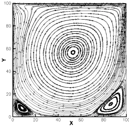
The LBM code is written and validated using lid driven cavity problem with Reynolds number of 1000. The 101×101 lattices in a square cavity with a moving lid and three fixed walls shows a good agreement with previous works [10-13].
[image:2.595.321.545.520.738.2]The streamlines are presented in Fig. 2. There are two secondary vortexes in lower right and left and one primary vortex in the center. Center positions of these three vortexes are reported on Table I. As a consequence of this table the difference of present work and Ghia et al. [10] in the center position of primary, lower left and lower right are 0.6, 5 and 2.1 percents, respectively.
TABLEI
COMPARISON OF THREE VORTEXES COORDINATION OF LID-DRIVEN CAVITY AT RE=1000(FIG.2)
Primary Vortex
Lower left Vortex
Lower right Vortex X Y X Y X Y
Present work 0.5310 0.5663 0.0818 0.0782 0.8631 0.1117
Ghia [10] 0.5313 0.5625 0.0859 0.0781 0.8594 0.1094
Schreiber [11] 0.5286 0.5643 0.0857 0.0714 0.8643 0.1071
Venka [12] 0.5438 0.5625 0.0750 0.0813 0.8625 0.1063
Hou [13] 0.5333 0.5647 0.0902 0.0784 0.8667 0.1137
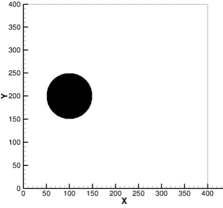
[image:3.595.340.498.63.746.2]Lattice Boltzmann method is weakly compressible approximation of incompressible Navier-Stokes equations. Its error is of order of Ma2 and can be neglected in pressure or density gradient of 10% [14]. In this study, a square with 401×401 nodes in D2Q9 lattice is used. The domain is at rest with the density of 1. A circle source with diameter of 100 nodes and density of 1.1 is on position of (100,200) at start time of simulation. The relaxation time is assumed to be 1. The geometry and initial source is illustrated in Fig.3.
Fig. 3. Circular source in a square domain at initial time
( 1.1, 1)
black white
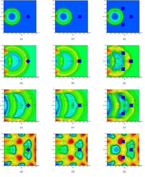
In order to see the propagation of the source and its interaction with solid boundaries four different scenarios are tested. The first test is simulated with no block and subsequently a 40×40 square rotated block at (300,200). At the third scenario, a 40×40 square block at (300,200) and the last scenario is three 40×40 square blocks which are positioned at (300,200), (200,100) and (200,300).
(a)
(b)
(c)
(d)
[image:3.595.59.287.404.616.2](a) (a) (a)
(b) (b) (b)
(c) (c) (c)
[image:4.595.59.534.66.644.2](d) (d) (d)
Fig. 5. Contour of density in scenario (2) at time step: a) 100, b) 250, c) 350, d) 500
Fig. 6. Contour of density in scenario (3) at time step: a) 100, b) 250, c) 350, d) 500
Fig. 7. Contour of density in scenario (4) at time step: a) 100, b) 250, c) 350, d) 500
The wave propagates with time. Density contours of domain are presented in Fig. 4 to 7 in time steps of 100, 250, 350 and 500 (a, b, c, d). In Fig. 4-a to 7-a which are at time step of 100 the left side of the wave front touches the left wall and reflects back. High-density zone can be observed in this region. They are same in four scenarios and blocks don’t affect the wave yet. In Fig. 5-b to 7-b the right side of
high density wave reaches to and reflects from the blocks on (300,200) in Fig. 5-b to 7-b and right wall in Fig. 4-d to 7-d and is recognizable with its high density value in contours. Its left front decomposes to two high-density zones and reflects from the left wall to right side. They are in the centerline of domain at time step 500. A low-density zone in the left side of these two high-density zones can be seen. The shape of this low-density zone is more circular in Fig. 7-d than other scenarios because of the existence of two blocks on centerline, which prevent two high-density zones to pass rightward. The other difference which can be observed on the right wall is the shape of high density regions at time step 500. Although there are two sections in Fig. 4-d but positioning a block in Fig. 5-d and 6-d makes them three sections. In Fig. 7-d two regions of these high density zones are weakened because of two centerline blocks effect.
IV. CONCLUSION
Lattice Boltzmann method was used to study the wave propagation in a domain and its interaction with solid boundaries including blocks and walls. A numerical code was developed based on streaming and collision. The code was validated with a lid-driven square cavity with reported works and indicated a good agreement. Effect of position and shape of the blocks on the wave propagation were presented with contours. Comparison showed that effect of blocks on the right wave front is obvious also the tails of the wave fronts which were low density zones were affected by blocks. Therefore, Lattice Boltzmann modeling of wave propagation and reflection has the ability to simulate weakly compressible flows like acoustic waves.
REFERENCES
[1] U. Frisch, B. Hasslacher, Y. Pomeau, “Lattice gas automata for the Navier–Stokes equations”, Phys. Rev. Lett., Vol. 56, 1986, pp. 1505– 1508.
[2] G. McNamara, G. Zanetti, “Use of the Boltzmann equation to simulate lattice-gas automata”, Phys. Rev. Lett., vol 61, 1988, pp. 2332-2335.
[3] X. Shan, X. F. Yuan, H. Chen, “Kinetic theory representation of hydrodynamics: a way beyond the Navier–Stokes equation”, J. Fluid Mech., vol. 550, 2006, pp. 413- 441.
[4] C. K. Aidun, J. R. Clasusen, “Lattice-Boltzmann method for complex flows”, Annu. Rev. Fluid Mech., vol. 42, 2009, pp. 439-472. [5] S. Succi, “Lattice Boltzmann across scales: from turbulence to DNA
translocation”, Eur. Phys. J. B., vol. 64, 2008, pp. 471–479. [6] E. M. Viggen, “The lattice Boltzmann method with applications in
acoustics”, MSc Thesis, Dept. of Physics, NTNU, Norway, 2009. [7] J. A. Cosgrove, J. M. Buick, D. M. Campbell, C. A. Greated,
“Numerical simulation of particle motion in an ultrasound field using the lattice Boltzmann model”, Ultrasonics, vol. 43, 2004, pp. 21-25. [8] D. Ricot, S. Marie, P. Sagaut, C. Bailly, “Lattice Boltzmann method
with selective viscosity filter”, J. Comp. Phys., vol. 228, 2009, pp. 4478–4490.
[9] J. M. Buick, C. L. Buckley, C. A. Greated, J. Gilbert, “Lattice Boltzmann BGK simulation of nonlinear sound waves: the development of a shock front”, J. Phys. A., vol. 33, 2000, pp. 3917-3928.
[10] K. N. Ghia, U. Ghia and C. T. Shin “High-Resolutions for incompressible flow using the Navier-Stokes equations and a multigrid method”, J. Comp. Phys., vol. 48, 1982, pp. 387-411. [11] R. Schreiber, H. B. Keller, “Driven cavity flows by efficient
numerical techniques”, J. Comp. Phys., vol. 49, 1983, pp. 310-333. [12] S. P. Vanka, “Block-implicit multigrid solution of Navier–Stokes
equations in primitive variables”, J. Comp. Phys., vol. 65, 1986, pp. 138–158.
[13] S. Hou and Q. Zou, S. Chen, G. Doolen, A. C. Cogley, “Simulation of Cavity Flow by the Lattice Boltzmann Method”, J. Comp. Phys., vol. 118, 1995, pp. 329-347.