645
Named Entity Recognition with Partially Annotated Training Data
Stephen Mayhew
\, Snigdha Chaturvedi
], Chen-Tse Tsai
[, Dan Roth
\ \University of Pennsylvania, Philadelphia, PA, 19104
]
University of North Carolina, Chapel Hill, NC, 27599
[
Bloomberg LP
{
mayhew, danroth
}
@seas.upenn.edu,
[email protected], [email protected]
Abstract
Supervised machine learning assumes the availability of fully-labeled data, but in many cases, such as low-resource languages, the only data available is partially annotated. We study the problem of Named Entity Recogni-tion (NER) with partially annotated training data in which a fraction of the named enti-ties are labeled, and all other tokens, entienti-ties or otherwise, are labeled as non-entity by default. In order to train on this noisy dataset, we need to distinguish between the true and false neg-atives. To this end, we introduce a constraint-driven iterative algorithm that learns to detect false negatives in the noisy set and downweigh them, resulting in a weighted training set. With this set, we train a weighted NER model. We evaluate our algorithm with weighted vari-ants of neural and non-neural NER models on data in 8 languages from several language and script families, showing strong ability to learn from partial data. Finally, to show real-world efficacy, we evaluate on a Bengali NER corpus annotated by non-speakers, outperforming the prior state-of-the-art by over 5 points F1.
1
Introduction
Most modern approaches to NLP tasks rely on super-vised learning algorithms to learn and generalize from labeled training data. While this has proven successful in high-resource scenarios, this is not realistic in many cases, such as low-resource languages, as the required amount of training data just doesn’t exist. However, partial annotations are often easy to gather.
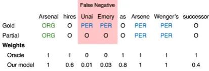
[image:1.595.312.519.250.320.2]We study the problem of using partial annotations to train a Named Entity Recognition (NER) system. In this setting, all (or most) identified entities are correct, but not all entities have been identified, and crucially, there are no reliable examples of the negative class. The sentence shown in Figure 1 shows examples of both a gold and a partially annotated sentence. Such partially annotated data is relatively easy to obtain: for
Figure 1: This example has three entities: Arsenal,
Unai Emery, andArsene Wenger. In thePartial row, the situation addressed in this paper, only the first and last are tagged, and all other tokens are assumed to be non-entities, making Unai Emerya false negative as compared toGold. Our model is an iteratively learned binary classifier used to assign weights to each token indicating its chances of being correctly labeled. The
Oraclerow shows optimal weights.
example, a human annotator who does not speak the target language may recognize common entities, but not uncommon ones. With no reliable examples of the negative class, the problem becomes one of estimating which unlabeled instances are true negatives and which are false negatives.
To address the above-mentioned challenge, we present Constrained Binary Learning (CBL) – a novel self-training based algorithm that focuses on iteratively identifying true negatives for the NER task while im-proving its learning. Towards this end, CBL uses constraints that incorporate background knowledge re-quired for the entity recognition task.
2
Related Work
The supervision paradigm in this paper, partial su-pervision, falls broadly under the category of semi-supervision (Chapelle et al.,2009), and is closely re-lated to weak supervision (Hern´andez-Gonz´alez et al.,
2016)1and incidental supervision (Roth,2017), in the sense that data is constructed through some noisy pro-cess. However, all of the most related work shares a key difference from ours: reliance on a small amount of fully annotated data in addition to the noisy data.
Fernandes and Brefeld(2011) introduces a transduc-tive version of structured perceptron for partially an-notated sequences. However, their definition of partial annotation is labels removed at random, so examples from all classes are still available if not contiguous.
Fidelity Weighted Learning (Dehghani et al.,2017) uses a teacher/student model, in which the teacher has access to (a small amount) of high quality data, and uses this to guide the student, which has access to (a large amount) of weak data.
Hedderich and Klakow (2018), following Gold-berger and Ben-Reuven(2017), add a noise adaptation layer on top of an LSTM, which learns how to correct noisy labels, given a small amount of training data. We compare against this model in our experiments.
In the world of weak supervision, Snorkel (Ratner et al.,2017;Fries et al.,2017), is a system that com-bines automatic labeling functions with data integra-tion and noise reducintegra-tion methods to rapidly build large datasets. They rely on high recall and consequent re-dundancy of the labeling functions. We argue that in certain realistic cases, high-recall candidate identifica-tion is unavailable.
We draw inspiration from the Positive-Unlabeled (PU) learning framework (Liu et al.,2002,2003;Lee and Liu,2003;Elkan and Noto,2008). Originally in-troduced for document classification, PU learning ad-dresses problems where examples of a single class (for example, sports) are easy to obtain, but a full labeling of all other classes is prohibitively expensive.
Named entity classification as an instance of PU learning was introduced inGrave(2014), which uses constrained optimization with constraints similar to ours. However, they only address the problem of named entity classification, in which mentions are given, and the goal is to assign atypeto a named-entity (like ‘location’, ‘person’, etc.) as opposed to our goal of identifying and typing named entities.
Although the task is slightly different, there has been work on building ‘silver standard’ data from Wikipedia (Nothman et al.,2008,2013; Pan et al.,2017), using hyperlink annotations as the seed set and propagating throughout the document.
Partial annotation in various forms has also been studied in the contexts of POS-tagging (Mori et al.,
1See also:https://hazyresearch.github.io/
snorkel/blog/ws_blog_post.html
2015), word sense disambiguation (Hovy and Hovy,
2012), temporal relation extraction (Ning et al.,2018), dependency parsing (Flannery et al.,2012), and named entity recognition (Jie et al.,2019).
In particular,Jie et al.(2019) study a similar problem with a few key differences: since they remove entity surfaces randomly, the dataset is too easy; and they do not use constraints on their output. We compare against their results in our experiments.
Our proposed method is most closely aligned with the Constraint Driven Learning (CoDL) framework (Chang et al.,2007), in which an iterative algorithm reminiscent of self-training is guided by constraints that are applied at each iteration.
3
Constrained Binary Learning
Our method assigns instance weights to all negative el-ements (tokens tagged as O), so that false negatives have low weights, and all other instances have high weights. We calculate weights according to the confi-dence predictions of a classifier trained iteratively over the partially annotated data. We refer to our method as Constrained Binary Learning (CBL).2
We will first describe the motivation for this ap-proach before moving on to the mechanics. We start with partially annotated data (which we call setT) in which some, but not all, positives are annotated (setP), and no negative is labeled. By default, we assume that any instance not labeled as positive is labeled as nega-tive as opposed to unlabeled. This data (setN) is noisy in the sense that many true positives are labeled as neg-ative (these arefalse negatives). Clearly, training onT as-is will result in a noisy classifier.
Two possible approaches are:1)find the false nega-tives and label them correctly, or2)find the false neg-atives and remove them. The former method affords more training data, but runs the risk of adding noise, which could be worse than the original partial annota-tions. The latter is more forgiving because of an asym-metry in the penalties: it is important to remove all false negatives inN, but inadvertently removing true nega-tives fromN is typically not a problem, especially in NER, where negative examples dominate. Further, a binary model (only two labels) is sufficient in this case, as we need only detect entities, not type them.
We choose the latter method, but instead of remov-ing false negatives, we adopt an instance-weightremov-ing ap-proach, in which each instance is assigned a weight vi ≥0according to confidence in the labeling of that
instance. A weight of0means that the loss this instance incurs during training will not update the model.
With this in mind, CBL takes two phases: first, it learns a binary classifierλusing a constrained iterative process modeled after the CODL framework (Chang et al., 2007), and depicted in Figure2. The core of
2Publication details (including code) can be found at
Require:
P : positive tokens N : noisy negative tokens C: constraints
1: T =N∪P
2: V ←InitializeT with weights (Optional)
3: whilestopping condition not metdo
4: λ←train(T, V)
5: Tˆ←predict(λ, T)
6: T, V ←inference( ˆT , C)
7: end while
8: returnλ
Figure 2: Constrained Binary Learning (CBL) algo-rithm (phase 1). The core of the algoalgo-rithm is in the while loop, which iterates over training onT, predict-ing onTand correcting those predictions.
the algorithm is the predict-infer loop. The train-ing process (line 4) is weighted, ustrain-ing weightsV. At the start, these can be all 1 (Raw), or can be initialized with prior knowledge. The learned model is then used to predict on all ofT(line 5). In the inference step (line 6), we take the predictions from the prior round and the constraintsCand produce a new labeling onT, and a new set of weightsV. The details of this inference step are presented later in this section. Although our ulti-mate strategy is simply to assign weights (not change labels), in this inner loop, we update the labels onN according to classifier predictions.
In the second phase of CBL, we use the λtrained in the previous phase to assign weights to instances as follows:
vi= (
1.0 ifxi∈P Pλ(yi=O|xi) ifxi∈N
(1)
WherePλ(yi = O | xi)is understood as the
clas-sifier’s confidence that instancexi takes the negative
label. In practice it is sufficient to use any confidence score from the classifier, not necessarily a probability. If the classifier has accurately learned to detect entities, then for all the false negatives inN,Pλ(yi =O|xi)is
small, which is the goal.
Ultimately, we send the original multiclass partially annotated dataset along with final weightsV to a stan-dard weighted NER classifier to learn a model. No weights are needed at test time.
3.1 NER with CBL
So far, we have given a high-level view of the algo-rithm. In this section, we will give more low-level de-tails, especially as they relate to the specific problem of NER. One contribution of this work is the inference step (line 6), which we address using a constrained In-teger Linear Program (ILP) and describe in this section. However, the constraints are based on a value we call theentity ratio. First, we describe the entity ratio, then
we describe the constraints and stopping condition of the algorithm.
3.1.1 Entity ratio and Balancing
We have observed that NER datasets tend to hold a rel-atively stable ratio of entity tokens to total tokens. We refer to this ratio asb, and define it with respect to some labeled dataset as:
b= |P|
|P|+|N| (2)
whereN is the set of negative examples. Previous work has shown that in fully-annotated datasets the en-tity ratio tends to be about0.09±0.05, depending on the dataset and genre (Augenstein et al.,2017). Intu-itively, knowledge of the gold entity ratio can help us estimate when we have found all the false negatives.
In our main experiments, we assume that the en-tity ratio with respect to the gold labeling is known for each training dataset. A similar assumption was made inElkan and Noto(2008) when determining the cvalue, and inGrave(2014) in the constraint determin-ing the percentage ofOTHER examples. However, we also show in Section4.8that knowledge of this ratio is not strictly necessary, and a flat value across all datasets produces similar performance.
With a weighted training set, it is also useful to de-fine the weighted entity ratio.
b= |P|
|P|+P i∈Nvi
(3)
When training an NER model on weighted data, one can change the weighted entity ratio to achieve differ-ent effects. To make balanced predictions on test, the entity ratio in the training data should roughly match that of the test data (Chawla,2005). To bias a model to-wards predicting positives or predicting negatives, the weighted entity ratio can be set higher or lower respec-tively. This effect is pronounced when using linear methods for NER, but not as clear in neural methods.
To change the entity ratio, we scale the weights inN by a scaling constantγ. Targeting a particularb∗, we may write:
b∗= |P|
|P|+γP i∈Nvi
(4)
We can solve forγ:
γ= (1−b
∗)|P|
b∗P i∈Nvi
(5)
To obtain weights,vi∗, that attain the desired entity ratio,b∗, we scale all weights inNbyγ.
vi∗=γvi (6)
3.1.2 Constraints and Stopping Condition
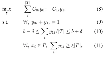
We encode our constraints with an Integer Linear Pro-gram (ILP), shown in Figure3. Intuitively, the job of the inference step is to take predictions (Tˆ) and use knowledge of the task to ‘fix’ them.
In the objective function (Eqn. 8), tokeniis repre-sented by two indicator variablesy0iandy1i,
represent-ing negative and positive labels, respectively. Associ-ated prediction scoresC0andC1are from the classifier
λin the last round of predictions. The first constraint (Eqn. 9) encodes the fact that an instance cannot be both an entity and a non-entity.
The second constraint (Eqn.10) enforces the ratio of positive to total tokens in the corpus to match a required entity ratio. |T| is the total number of tokens in the corpus.bis the required entity ratio, which increases at each iteration.δallows some flexibility, but is small.
Constraint11encodes that instances inPshould be labeled positive since they were manually labeled and are by definition trustworthy. We setξ≥0.99.
This framework is flexible in that more complex language- or task-specific constraints could be added. For example, in English and many other languages with Latin script, it may help to add a capitalization con-straint. In languages with rich morphology, certain suf-fixes may indicate or contraindicate a named entity. For simplicity, and because of the number of languages in our experiments, we use only a few constraints.
After the ILP has selected predictions, we assign weights to each instance in preparation for training the next round. The decision process for an instance is:
vi= (
1.0 If ILP labeledxipositive Pλ(yi=O|xi) Otherwise
(7) This is similar to Equation (1), except that the set of tokens that the ILP labeled as positive is larger thanP. With new labels and weights, we start the next iteration. The stopping condition for the algorithm is related to the entity ratio. One important constraint (Eqn.
10) governs how many positives are labeled at each round. This number starts at|P| and is increased by a small value3at each iteration, thereby improving re-call. Positive instances are chosen in two ways. First, all instances inPare constrained to be labeled positive (Eqn. 11). Second, the objective function ensures that high-confidence positives will be chosen. The stopping condition is met when the number of required positive instances (computed using gold unweighted entity ra-tio) equals the number of predicted positive instances.
4
Experiments
We measure the performance of our method on 8 dif-ferent languages using artificially perturbed labels to
3The size of this value is related to how much we trust the
ranking induced by prediction confidences. If we believed the ranking was perfect, we could take as many positives as we wanted and be finished in one round.
max
y
|T|
X
i
C0iy0i+C1iy1i (8)
s.t. ∀i, y0i+y1i= 1 (9)
b−δ≤X
i
y1i/|T| ≤b+δ (10)
∀i, xi∈P, X
i
[image:4.595.326.526.73.183.2]y1i≥ξ|P|, (11)
Figure 3: ILP for the inference step
simulate the partial annotation setting.
4.1 Data
We experiment on 8 languages. Four languages – English, German, Spanish, Dutch – come from the CoNLL 2002/2003 shared tasks (Tjong Kim Sang and De Meulder,2003a,b). These are taken from newswire text, and have labelset of Person, Organization, Loca-tion, Miscellaneous.
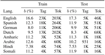
The remaining four languages come from the LORELEI project (Strassel and Tracey,2016). These languages are: Amharic (amh: LDC2016E87), Arabic (ara: LDC2016E89), Hindi (hin: LDC2017E62), and Somali (som: LDC2016E91). These come from a vari-ety of sources including discussion forums, newswire, and social media. The labelset is Person, Orga-nization, Location, Geo-political entity. We define train/development/test splits, taking care to keep a sim-ilar distribution of genres in each split. Data statistics for all languages are shown in Table1.
4.2 Artificial Perturbation
We create partial annotations by perturbing gold anno-tated data in two ways: lowering recall (to simulate missing entities), and lowering precision (to simulate noisy annotations).
To lower recall, we replace gold named entity tags withOtags (for non-name). We do this by grouping named entity surface forms, and replacing tags on all occurrences of a randomly selected surface form until the desired amount remains. For example, if the to-ken ‘Bangor’ is chosen to be untagged, then every oc-currence of ‘Bangor’ will be untagged. We chose this slightly complicated method because the simplest idea (remove mentions randomly) leaves an artificially large diversity of surface forms, which makes the problem of discovering noisy entities easier.
To lower precision, we tag a random span (of a ran-dom start position, and a ranran-dom length between1and
Train Test Lang. b(%) Tag Tok b(%) Tag Tok English 16.6 23K 203K 17.3 5K 46K Spanish 12.3 18K 264K 11.9 3K 51K German 8.0 11K 206K 9.9 3K 51K Dutch 9.5 13K 202K 8.3 4K 68K Amharic 11.2 3K 52K 11.3 1K 18K Arabic 12.6 4K 60K 10.2 931 16K Hindi 7.38 4K 74K 7.53 1K 25K Somali 11.2 4K 57K 11.9 1K 16K
Table 1: Data statistics for all languages, showing num-ber of tags and tokens in Train and Test. The tag counts represent individual spans, not tokens. That is, “[Barack Obama]PER” counts as one tag, not two. The
bcolumn shows the entity ratio as a percentage.
4.3 NER Models
In principle, CBL can use any NER method that can be trained with instance weights. We experiment with both non-neural and neural models.
4.3.1 Non-neural Model
For our non-neural system, we use a version of Cog-comp NER (Ratinov and Roth,2009;Khashabi et al.,
2018) modified to use Weighted Averaged Percep-tron. This operates on a weighted training setDw =
{(xi, yi, vi)}Ni=1, where N is the number of training
examples, andvi ≥0is the weight on theith training
example. In this non-neural system, a training exam-ple is a word with context encoded in the features. We change only the update rule, where the learning rateα is multiplied by the weight:
w=w+αviyi(wTxi) (12)
We use a standard set of features, as documented in Ratinov and Roth (2009). In order to keep the language-specific resources to a minimum, we did not use any gazetteers for any language.4 One of the most important features is Brown clusters, trained for 100, 500, and 1000 clusters for the CoNLL languages, and 2000 clusters for the remaining languages. We trained these clusters on Wikipedia text for the four CoNLL languages, and on the same monolingual text used to train the word vectors (described in Section4.3.2).
4.3.2 Neural Model
A common neural model for NER is the BiLSTM-CRF model (Ma and Hovy, 2016). However, because the Conditional Random Field (CRF) layer calculates loss at the sentence level, we need a different method to in-corporate token weights. We use a variant of the CRF that allows partial annotations by marginalizing over all possible sequences (Tsuboi et al.,2008).
4Separate experiments show that omitting gazetteers
im-pacts performance only slightly.
When using a standard BiLSTM-CRF model, the loss of a dataset (D) composed of sentences (s) is cal-culated as:
L=−X
s∈D
logPθ(y(s)|x(s)) (13)
WherePθ(y(s)|x(s))is calculated by the CRF over
outputs from the BiLSTM. In the marginal CRF frame-work, it is assumed thaty(s)is necessarily partial,
de-noted asy(ps). To incorporate partial annotations, the
loss is calculated by marginalizing over all possible sequences consistent with the partial annotations, de-noted asC(ys
p).
L=−X
s∈D
log X
y∈C(y(ps))
Pθ(y|x(s)) (14)
However, this formulation assumes that all possible sequences are equally likely. To address this,Jie et al.
(2019) introduced a way to weigh sequences.
L=−X
s∈D
log X
y∈C(y(ps))
q(y|x(s))P
θ(y|x(s)) (15)
It’s easy to see that this formulation is a generaliza-tion of the standard CRF ifq(.) = 1for the gold se-quencey, and 0 for all others.
The product inside the summation depends on tag transition probabilities and tag emission probabilities, as well as token-level “weights” over the tagset. These weights can be seen as defining a soft gold labeling for each token, corresponding to confidence in each label.
For clarity, define the soft gold labeling over each tokenxi as Gi ∈ [0,1]L, whereL is the size of the
labelset. Now, we may defineq(.)as:
q(y|x(s)) =Y i
Gyi
i
WhereGyi
i is understood as the weight inGi that
corresponds to the labelyi.
We incorporate our instance weights in this model with the following intuitions. Recall that if an instance weightvi= 0, this indicates low confidence in the label
on tokenxi, and therefore the labeling should not
up-date the model at training time. Conversely, ifvi = 1,
then this label is to be trusted entirely.
Ifvi= 0, we set the soft labeling weights overxito
be uniform, which is as good as no information. Since vi is defined as confidence in the O label, the soft
la-beling weight for O increases proportionally tovi. Any
remaining probability mass is distributed evenly among the other labels.
To be precise, for tokens inN, we calculate values forGias follows:
GOi = max(1/L, vi)
Gnon-i O=
For example, consider phase 1 of Constrained Binary Learning, in which the labelset is collapsed to two la-bels (L= 2). Assuming that the O label has index 0, then ifvi = 0, thenGi = [0.5,0.5]. Ifvi = 0.6, then
Gi= [0.6,0.4].
For tokens inP (which have some entity label with high confidence), we always setGiwith 1 in the given
label index, and 0 elsewhere.
We use pretrained GloVe (Pennington et al., 2014) word vectors for English, and the same pretrained vec-tors used in Lample et al.(2016) for Dutch, German, and Spanish. The other languages are distributed with monolingual text (Strassel and Tracey, 2016), which we used to train our own skip-n-gram vectors.
4.4 Baselines
We compare against several baselines, including two from prior work.
4.4.1 Raw annotations
The simplest baseline is to do nothing to the partially annotated data and train on it as is.
4.4.2 Instance Weights
Although CBL works with no initialization (that is, all tokens with weight 1), we found that a good weight-ing scheme can boost performance for certain models. We design weighting schemes that give instances inN weights corresponding to an estimate of the label con-fidence.5 For example, non-name tokens such as
re-spectfully should have weight 1, but possible names, such asRussell, should have a low weight, or 0. We propose two weighting schemes: frequency-based and window-based.
For the frequency-based weighting scheme, we ob-served that names have relatively low frequency (for example, Kennebunkport, Dushanbe) and common words are rarely names (for examplethe,and,so). We weigh each instance inN according to its frequency.
vfreqi =f req(xi) (16)
wheref req(xi)is the frequency of theithtoken in N divided by the count of the most frequent token. In our experiments, we computed frequencies overP+N, but these could be estimated on any sufficiently large corpus. We found that the neural model performed poorly when the weights followed a Zipfian distribu-tion (e.g. most weights very small), so for those ex-periments, we took the log of the token count before normalizing.
For the window-based weighting scheme, noting that names rarely appear immediately adjacent to each other in English text, we set weights for tokens within a win-dow of size 1 of a name (identified inP) to be1.0, and for tokens farther away to be0.
viwindow= (
1.0 ifdi ≤1
0.0 otherwise (17)
5All elements ofPalways have weight 1
wherediis the distance of theithtoken to the nearest
named entity inP.
Finally, we combine the two weighting schemes as:
vcombinedi = (
1.0 ifdi≤1
vfreqi otherwise (18)
4.4.3 Self-training with Marginal CRF
Jie et al.(2019) propose a model based on marginal CRF (Tsuboi et al.,2008) (described in Section4.3.2). They follow a self-training framework with cross-validation, using the trained model over all but one fold to update gold labeling distributions in the final fold. This process continues until convergence. They use a partial-CRF framework similar to ours, but taking pre-dictions at face value, without constraints.
4.4.4 Neural Network with Noise Adaptation
Following Hedderich and Klakow(2018), we used a neural network with a noise adaptation layer.6 This extra layer attempts to correct noisy examples given a probabilistic confusion matrix of label noise. Since this method needs a small amount of labeled data, we selected 500 random tokens to be the gold training set, in addition to the partial annotations.
As with our BiLSTM experiments, we use pretrained GloVe word vectors for English, and the same pre-trained vectors used inLample et al.(2016) for Dutch, German, and Spanish. We omit results from the re-maining languages because the scores were substan-tially worse even than training on raw annotations.
4.5 Experimental Setup and Results
We show results from our experiments in Table2. In all experiments, the training data is perturbed at 90% precision and 50% recall. These parameters are similar to the scores obtained by human annotators in a foreign language (see Section5). We evaluate each experiment with both non-neural and neural methods.
First, to get an idea of the difficulty of NER in each language, we report scores from models trained on gold data without perturbation (Gold). Then we re-port results from an Oracle Weighting scheme ( Ora-cle Weighting) that takes partially annotated data and assigns weights with knowledge of the true labels. Specifically, mislabeled entities in set N are given weight 0, and all other tokens are given weight 1.0. This scheme is free from labeling noise, but should still get lower scores than Gold because of the smaller number of entities. Since our method estimates these weights, we do not expect CBL to outperform the Or-acle method. Next, we show results from all baselines. The bottom two sections are our results, first with no initialization (Raw), and CBL over that, then with Com-bined Weightinginitialization, and CBL over that.
Method\Language Tool eng deu esp ned amh ara hin som avg
Gold Cogcomp 89.1 72.5 82.5 82.6 67.2 53.4 74.4 80.3 75.3 BiLSTM-CRF 90.3 77.3 85.2 81.1 69.2 52.8 73.8 82.3 76.5
Oracle Weighting Cogcomp 83.7 65.7 76.2 76.4 54.3 42.0 56.3 68.5 65.4 BiLSTM-CRF 87.8 70.2 78.5 70.4 60.4 43.4 57.6 73.2 67.7
Noise Adaptation(Hedderich, 2018) 61.5 46.1 57.3 41.5 – – – – – Self-training (Jie et al.,2019) 82.3 65.2 76.3 65.5 52.1 40.1 55.1 65.3 62.7
Raw Annotations Cogcomp 54.8 36.9 49.5 47.9 31.0 32.6 30.9 44.0 40.9 BiLSTM-CRF 73.3 57.7 61.9 58.3 42.2 36.8 47.5 54.9 54.1
CBL-Raw CogComp 74.7 63.0 68.7 67.0 45.0 37.8 50.6 67.9 59.3 BiLSTM-CRF 84.6 67.9 79.6 70.0 52.9 42.1 55.2 70.4 65.3
Combined Weighting Cogcomp 75.2 56.6 70.8 70.8 46.5 44.1 57.5 60.2 60.2 BiLSTM-CRF 73.5 60.3 64.9 61.9 48.0 38.0 49.0 56.6 56.5
[image:7.595.82.516.64.273.2]CBL-Combined Cogcomp 77.3 61.8 74.0 72.4 49.2 43.7 58.2 67.6 63.0 BiLSTM-CRF 81.1 64.9 74.9 63.4 52.2 39.8 52.0 67.0 61.9
Table 2: F1 scores on English, German, Spanish, Dutch, Amharic, Arabic, Hindi, and Somali. Each section shows performance of both Cogcomp (non-neural) and BiLSTM (neural) systems.Goldis using all available gold training data to train. Oracle Weightinguses full entity knowledge to set weights onN. The next section shows prior work, followed by our methods. The column to the farthest right shows the average score over all languages. Bold values are the highest per column. On average, our best results are found in the uninitialized (Raw) CBL from BiLSTM-CRF.
4.6 Analysis
Regardless of initialization or model, CBL improves over the baselines. Our best model,CBL-Raw BiLSTM-CRF, improves over the Raw Annotations BiLSTM-CRFbaseline by 11.2 points F1, and theSelf-training
prior work by 2.6 points F1, showing that it is an effec-tive way to address the problem of partial annotation. Further, the best CBL version for each model is within 3 points of the correspondingOracleceiling, suggest-ing that this weightsuggest-ing framework is nearly saturated.
TheCombinedweighting scheme is surprisingly ef-fective for the non-neural model, which suggests that the intuition about frequency as distinction between names and non-names holds true. It gives modest improvement in the neural model. The Self-training
method is effective, but is outperformed by our best CBL method, a difference we discuss in more detail in Section4.7. TheNoise Adaptationmethod outper-forms theRaw annotations Cogcompbaseline in most cases, but does not reach the performance of the Self-trainingmethod, despite using some fully labeled data.
It is instructive to compare the neural and non-neural versions of each setup. The neural method is better overall, but is less able to learn from the knowledge-based initialization weights. In the non-neural method, the difference between Raw andCombined is nearly 20 points, but the difference in the neural model is less than 3 points. Combined versions of the non-neural method outperform the non-neural method on 3 lan-guages: Dutch, Arabic, and Hindi. Further, in the neural method, CBL-Rawis always worse than
CBL-Combined. This may be due to the way that weights are used in each model. In the non-neural model, a low enough weight completely cancels the token, whereas in the neural model it is still used in training. Since the neural model performs well in theOracle setting, we know that it can learn from hard weights, but it may have trouble with the subtle differences encoded in frequencies. We leave it to future work to discover improved ways of incorporating instance weights in a BiLSTM-CRF.
In seeking to understand the details of the other re-sults, we need to consider the precision/recall tradeoff. First, all scores in theGold row had higher precision than recall. Then, training on raw partially annotated data biases a classifier strongly towards predicting few entities. All results from theRaw annotationsrow have precision more than double the recall (e.g. Dutch Preci-sion, Recall, F1 were: 91.5, 32.4, 47.9). In this context, the problem this paper explores is how to improve the recall of these datasets without harming the precision.
4.7 Difference from Prior Work
While our method has several superficial similarities with prior work, most notablyJie et al. (2019), there are some crucial differences.
Our methods are similar in that they both use a model trained at each step to assign a soft gold-labeling to each token. Each algorithm iteratively trains models using weights from the previous steps.
Avg F1
Method\b 10% 15% Gold
Oracle Weighting 65.8 65.9 65.4 Raw annotations 40.9 40.9 40.9 Combined Weighting 59.9 60.2 60.2
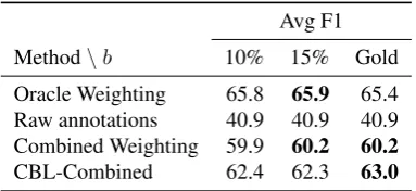
[image:8.595.86.278.62.150.2]CBL-Combined 62.4 62.3 63.0
Table 3: Experimenting with different entity ratios. Scores reported are average F1 across all languages.
Gold b value refers to using the gold annotated data to calculate the optimal entity ratio. This table shows that exact knowledge of the entity ratio is not required for CBL to succeed.
However, the main difference has to do with the fo-cus of each algorithm. Recall the disfo-cussion in Sec-tion3regarding the two possible approaches of1) find the false negatives and label them correctly, and2) find the false negatives and remove them. Conceptually, the former was the approach taken byJie et al.(2019), the latter was our approach. Another way to look at this is as focusing on predicting correct tag labels ((Jie et al.,
2019)) or focus on predicting O tags with high confi-dence (ours).
Even though they use soft labeling (which they show to be consistently better than hard labeling), it is possi-ble that the predicted tag distribution is incorrect. Our approach allows us to avoid much of the inevitable noise that comes from labelling with a weak model.
4.8 Varying the Entity Ratio
Recall that the entity ratio is used for balancing and for the stopping criteria in CBL. In all our experiments so far, we have used the gold entity ratio for each lan-guage, as shown in Table 1. However, exact knowl-edge of entity ratio is unlikely in the absence of gold data. Thus, we experimented with selecting a defaultb value, and using it across all languages, with the Cog-comp model. We chose values of10%and15%, and report F1 averaged across all languages in Table3.
While the gold b value is the best for CBL-Combined, the flat 15% ratio is best for all other meth-ods, showing that exact knowledge of the entity ratio is not necessary.
5
Bengali Case Study
So far our experiments have shown effectiveness on artificially perturbed labels, but one might argue that these systematic perturbations don’t accurately simu-late real-world noise. In this section, we show how our methods work in a real-world scenario, using Bengali data partially labeled by non-speakers.
5.1 Non-speaker Annotations
In order to compare with prior work, we used the train/test split fromZhang et al.(2016). We removed
Num tokens 49K
Num sentences 2435 Num name tokens 2326 Entity ratio 4.66% Num unique name tokens 664 Annotator 1 Prec/Rec/F1 84/34/48 Annotator 2 Prec/Rec/F1 79/28/42 Combined Prec/Rec/F1 83/32/47
Table 4: Bengali Data Statistics. The P/R/F1 scores are computed for the non-speaker annotator with respect to the gold training data.
all gold labels from the train split, romanized it7(
Her-mjakob et al., 2018), and presented it to two non-Bengali speaking annotators using the TALEN inter-face (Mayhew and Roth,2018). The instructions were to move quickly and annotate names only when there is high confidence (e.g. when you can also identify the English version of the name). They spent about 5 total hours annotating, without using Google Trans-late. This sort of non-speaker annotation is possible because the text contains many ‘easy’ entities – foreign names – which are noticeably distinct from native Ben-gali words. For example, consider the following:
• Romanized Bengali: ebisi’ra giliyyaana phinnd-dale aaja pyaalestaaina adhiinastha gaajaa theke aaja raate ekhabara jaaniyyechhena .
• Translation8: ABC’s Gillian Fondley has re-ported today from Gaza under Palestine today.
The entities are Gillian Findlay, ABC, Palestine, and Gaza. While a fast-moving annotator may not catch most of these, ‘pyaalestaaina’ could be considered an ‘easy’ entity, because of its visual and aural similarity to ‘Palestine.’ A clever annotator may also infer that if Palestine is mentioned, then Gaza may be present.
Annotators are moving fast and being intentionally non-thorough, so the recall will be low. Since they do not speak Bengali, there are likely to be some mistakes, so the precision may drop slightly also. This is exactly the noisy partial annotation scenario addressed in this paper. The statistics of this data can be seen in Table4, including annotation scores computed with respect to the gold training data for each annotator, as well as the combined score.
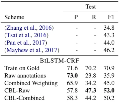
We show results in Table5, using the BiLSTM-CRF model. We compare against other low-resource ap-proaches published on this dataset, including two based on Wikipedia (Tsai et al.,2016;Pan et al.,2017), an-other based on lexicon translation from a high-resource language (Mayhew et al., 2017). These prior meth-ods operate under somewhat different paradigms than
7
This step is vitally important. We usedwww.isi.edu/ ˜ulf/uroman.html
[image:8.595.339.496.63.165.2]Test
Scheme P R F1
(Zhang et al.,2016) - - 34.8 (Tsai et al.,2016) - - 43.3 (Pan et al.,2017) - - 44.0 (Mayhew et al.,2017) - - 46.2
BILSTM-CRF
Train on Gold 71.6 70.2 70.9 Raw annotations 73.0 23.8 35.9 Combined Weighting 65.9 34.2 45.0
CBL-Raw 57.8 47.3 52.0
[image:9.595.86.278.61.226.2]CBL-Combined 58.3 44.2 50.2
Table 5: Bengali manual annotation results. Our meth-ods improve on state of the art scores by over 5 points F1 given a relatively small amount of noisy and incom-plete annotations from non-speakers.
this work, but have the same goal: maximizing perfor-mance in the absence of gold training data.
Raw annotationsis defined as before, and gives sim-ilar high-precision low-recall results. The Combined Weightingscheme improves over Raw annotations by 10 points, achieving a score comparable to the prior state of the art. Beyond that, CBL-Rawoutperforms the prior best by nearly 6 points F1, although CBL-Combinedagain underwhelms.
To the best of our knowledge, this is the first result showing a method for non-speaker annotations to pro-duce high-quality NER scores. The simplicity of this method and the small time investment for these results gives us confidence that this method can be effective for many low-resource languages.
6
Conclusions
We explore an understudied data scenario, and intro-duce a new constrained iterative algorithm to solve it. This algorithm performs well in experimental trials in several languages, on both artificially perturbed data, and in a truly low-resource situation.
7
Acknowledgements
This work was supported by Contracts HR0011-15-C-0113 and HR0011-18-2-0052 with the US Defense Ad-vanced Research Projects Agency (DARPA). Approved for Public Release, Distribution Unlimited. The views expressed are those of the authors and do not reflect the official policy or position of the Department of Defense or the U.S. Government.
References
Isabelle Augenstein, Leon Derczynski, and Kalina Bontcheva. 2017. Generalisation in named entity recognition: A quantitative analysis. Computer Speech and Language, 44:61–83.
M. Chang, L. Ratinov, and D. Roth. 2007. Guiding semi-supervision with constraint-driven learning. In
Proc. of the Annual Meeting of the Association for Computational Linguistics (ACL), pages 280–287, Prague, Czech Republic. Association for Computa-tional Linguistics.
Olivier Chapelle, Bernhard Scholkopf, and Alexander Zien. 2009. Semi-supervised learning (chapelle, o. et al., eds.; 2006)[book reviews]. IEEE Transactions on Neural Networks, 20(3):542–542.
Nitesh V. Chawla. 2005. Data mining for imbalanced datasets: An overview. In The Data Mining and Knowledge Discovery Handbook.
Mostafa Dehghani, Arash Mehrjou, Stephan Gouws, Jaap Kamps, and Bernhard Sch¨olkopf. 2017. Fidelity-weighted learning.CoRR, abs/1711.02799.
Charles Elkan and Keith Noto. 2008. Learning clas-sifiers from only positive and unlabeled data. In
Proceedings of the 14th ACM SIGKDD international conference on Knowledge discovery and data min-ing, pages 213–220. ACM.
Eraldo Rezende Fernandes and Ulf Brefeld. 2011. Learning from partially annotated sequences. In
ECML/PKDD.
Daniel Flannery, Yusuke Miyao, Graham Neubig, and Shinsuke Mori. 2012. A pointwise approach to training dependency parsers from partially anno-tated corpora.Information and Media Technologies, 7(4):1489–1513.
Jason A. Fries, Sen Wu, Alexander Ratner, and Christo-pher R´e. 2017. Swellshark: A generative model for biomedical named entity recognition without labeled data.CoRR, abs/1704.06360.
Jacob Goldberger and Ehud Ben-Reuven. 2017. Train-ing deep neural-networks usTrain-ing a noise adaptation layer. InICLR.
Edouard Grave. 2014. Weakly supervised named entity classification. InAKBC.
Michael A. Hedderich and Dietrich Klakow. 2018.
Training a neural network in a low-resource setting on automatically annotated noisy data. In Proceed-ings of the Workshop on Deep Learning Approaches for Low-Resource NLP, pages 12–18, Melbourne. Association for Computational Linguistics.
Jer´onimo Hern´andez-Gonz´alez, Inaki Inza, and Jose A Lozano. 2016. Weak supervision and other non-standard classification problems: a taxonomy. Pat-tern Recognition Letters, 69:49–55.
Dirk Hovy and Eduard Hovy. 2012. Exploiting partial annotations with EM training. InProceedings of the NAACL-HLT Workshop on the Induction of Linguis-tic Structure, pages 31–38, Montr´eal, Canada. Asso-ciation for Computational Linguistics.
Zhanming Jie, Pengjun Xie, Wei Lu, Ruixue Ding, and Linlin Li. 2019. Better modeling of incomplete an-notations for named entity recognition. In Proceed-ings of the 2019 Conference of the North American Chapter of the Association for Computational Lin-guistics: Human Language Technologies, Volume 1 (Long and Short Papers), pages 729–734, Min-neapolis, Minnesota. Association for Computational Linguistics.
Daniel Khashabi, Mark Sammons, Ben Zhou, Tom Redman, Christos Christodoulopoulos, Vivek Sriku-mar, Nicholas Rizzolo, Lev Ratinov, Guanheng Luo, Quang Do, Chen-Tse Tsai, Subhro Roy, Stephen Mayhew, Zhili Feng, John Wieting, Xiaodong Yu, Yangqiu Song, Shashank Gupta, Shyam Upadhyay, Naveen Arivazhagan, Qiang Ning, Shaoshi Ling, and Dan Roth. 2018.Cogcompnlp: Your swiss army knife for nlp. InLREC.
Guillaume Lample, Miguel Ballesteros, Sandeep Sub-ramanian, Kazuya Kawakami, and Chris Dyer. 2016.
Neural architectures for named entity recognition. InProceedings of the 2016 Conference of the North American Chapter of the Association for Computa-tional Linguistics: Human Language Technologies, pages 260–270, San Diego, California. Association for Computational Linguistics.
Wee Sun Lee and Bing Liu. 2003. Learning with posi-tive and unlabeled examples using weighted logistic regression. InICML.
Bing Liu, Yang Dai, Xiaoli Li, Wee Sun Lee, and Philip S. Yu. 2003. Building text classifiers using positive and unlabeled examples. InICDM.
Bing Liu, Wee Sun Lee, Philip S. Yu, and Xiaoli Li. 2002. Partially supervised classification of text doc-uments. InICML.
Xuezhe Ma and Eduard Hovy. 2016. End-to-end sequence labeling via bi-directional LSTM-CNNs-CRF. InProceedings of the 54th Annual Meeting of the Association for Computational Linguistics (Vol-ume 1: Long Papers), pages 1064–1074, Berlin, Germany. Association for Computational Linguis-tics.
Stephen Mayhew and Dan Roth. 2018. TALEN: Tool for annotation of low-resource ENtities. In Proceed-ings of ACL 2018, System Demonstrations, pages 80–86, Melbourne, Australia. Association for Com-putational Linguistics.
Stephen Mayhew, Chen-Tse Tsai, and Dan Roth. 2017.
Cheap translation for cross-lingual named entity recognition. InProc. of the Conference on Empirical Methods in Natural Language Processing (EMNLP).
Shinsuke Mori, Yosuke Nakata, Graham Neubig, and Tetsuro Sasada. 2015. Pointwise prediction and sequence-based reranking for adaptable part-of-speech tagging. InPACLING.
Qiang Ning, Zhongzhi Yu, Chuchu Fan, and Dan Roth. 2018. Exploiting partially annotated data in tempo-ral relation extraction. InProceedings of the Seventh Joint Conference on Lexical and Computational Se-mantics, pages 148–153, New Orleans, Louisiana. Association for Computational Linguistics.
Joel Nothman, James R Curran, and Tara Murphy. 2008. Transforming wikipedia into named entity training data. InProceedings of the Australian Lan-guage Technology Workshop, pages 124–132.
Joel Nothman, Nicky Ringland, Will Radford, Tara Murphy, and James R. Curran. 2013. Learning mul-tilingual named entity recognition from wikipedia.
Artif. Intell., 194:151–175.
Xiaoman Pan, Boliang Zhang, Jonathan May, Joel Nothman, Kevin Knight, and Heng Ji. 2017. Cross-lingual name tagging and linking for 282 languages. In Proceedings of the 55th Annual Meeting of the Association for Computational Linguistics (Volume 1: Long Papers), pages 1946–1958, Vancouver, Canada. Association for Computational Linguistics.
Jeffrey Pennington, Richard Socher, and Christopher Manning. 2014. Glove: Global vectors for word rep-resentation. InProceedings of the 2014 conference on empirical methods in natural language process-ing (EMNLP), pages 1532–1543.
L. Ratinov and D. Roth. 2009. Design challenges and misconceptions in named entity recognition. In
Proc. of the Conference on Computational Natural Language Learning (CoNLL).
Alexander Ratner, Stephen H. Bach, Henry R. Ehren-berg, Jason Alan Fries, Sen Wu, and Christopher R´e. 2017. Snorkel: Rapid training data creation with weak supervision. Proceedings of the VLDB Endow-ment. International Conference on Very Large Data Bases, 11 3:269–282.
Dan Roth. 2017. Incidental supervision: Moving be-yond supervised learning. InProc. of the Conference on Artificial Intelligence (AAAI).
Stephanie Strassel and Jennifer Tracey. 2016.
Erik F. Tjong Kim Sang and Fien De Meulder. 2003a. Introduction to the CoNLL-2003 shared task: Language-independent named entity recognition. In
Proceedings of the Seventh Conference on Natu-ral Language Learning at HLT-NAACL 2003, pages 142–147.
Erik F. Tjong Kim Sang and Fien De Meulder. 2003b. Introduction to the CoNLL-2003 shared task: Language-independent named entity recogni-tion. InProceedings of the Seventh Conference on Natural Language Learning at HLT-NAACL 2003, pages 142–147.
Chen-Tse Tsai, Stephen Mayhew, and Dan Roth. 2016.
Cross-lingual named entity recognition via wikifica-tion. InProc. of the Conference on Computational Natural Language Learning (CoNLL).
Yuta Tsuboi, Hisashi Kashima, Hiroki Oda, Shinsuke Mori, and Yuji Matsumoto. 2008. Training condi-tional random fields using incomplete annotations. InProceedings of the 22nd International Conference on Computational Linguistics-Volume 1, pages 897– 904. Association for Computational Linguistics.
Boliang Zhang, Xiaoman Pan, Tianlu Wang, Ashish Vaswani, Heng Ji, Kevin Knight, and Daniel Marcu. 2016. Name tagging for low-resource incident lan-guages based on expectation-driven learning. In