Abstract—Bone is a complex biological material due to its
heterogeneous and anisotropic nature. Finite element modeling (FEM) has been an effective tool in the field of bone mechanics to predict the behavior of bone material under different loading situations and the fracture locations. Bone exhibits different yield behavior along different material orientations due to its anisotropic nature and therefore for better understanding of bone behavior under multi-axial loading, it is necessary to incorporate anisotropic yielding and post yield properties in FEM. In the present study FE simulation of cortical bone was carried out using different yield stress ratios in different directions based on Hill’s criterion. Bone material was treated as a transversely isotropic material whose effective properties are isotropic in one of its planes. The tensile behavior of cortical bone in longitudinal and transverse directions was analyzed using two different uniaxial tensile models. The uniaxial tensile models were found to be in good agreement with the experimental results and therefore biaxial model of cortical bone was also developed and analyzed using the same approach. The study shows that Hill’s criterion gives good results for anisotropic yielding in bone material and can be used to simulate multidirectional loading situations in bone mechanics.
Index Terms— Anisotropic yielding, Cortical bone, Finite
element simulation, Transversely isotropic material
I. INTRODUCTION
ONE is a functionally graded material, composed by
hydroxyapatite, collagen, small amount of proteoglycans, non-collagenous proteins and water [1-4]. The multiphasic, heterogeneous and anisotropic microstructure of bone results in a very complex material type. Finite element modeling (FEM) has been a valuable tool for investigating a wide range of biological problems and widely used to study the behavior of bone in many clinical applications. Due to inhomogeneous and anisotropic nature of bone material it is quite difficult to specify its material properties for FE simulation. Therefore in various biological studies, bone is mostly modeled as linear elastic material [5-9]. However in limited studies researchers have
Manuscript received July 2, 2012.
N.K. Sharma is with the Indian Institute of Technology Delhi, Hauz Khas, New Delhi 110016, India (phone: +91-9310664161; e-mail: enksharma@ yahoo.com).
D. K. Sehgal is with the Indian Institute of Technology Delhi, Hauz Khas, New Delhi 110016, India (e-mail: [email protected]).
R. K. Pandey is with the Indian Institute of Technology Delhi, Hauz Khas, New Delhi 110016, India (e-mail: [email protected]).
Ruchita Paul is with the AIRF center, Jawaharlal Nehru University, New Delhi- 110067, India (e-mail: [email protected]).
obtained more accurate results by considering the non-linear material properties of cortical bone [10-11]. For the purpose of FE simulation in different studies of bone mechanics the mechanical properties of bone were predicted from computed tomographic (CT) numbers [12-15]. The mechanical properties of bone are related to its apparent density or ash density. The density of bone can be correlated to quantitative computed tomography (QCT) Hausfeld units (HU) resulting in Young’s modulus E-(HU) relationship but it is difficult to obtain various material properties of bone from a scalar value (HU) in QCT scans.
Although the investigation on multidimensional loading and its effect on bone material is very important as living bone is seldom loaded in one direction, due to complexity of loading it is difficult to experimentally obtain mechanical properties of bone under multiaxial loading. The FEM is considered to be used as an effective tool in this direction.
Bone as an anisotropic material exhibits different yield behavior in different directions. The present work is based on modeling of anisotropic yield behavior of cortical bone using yield stress ratios. In this study bone material is considered as a transversely isotropic material with five independent elastic constants. The long axis of the bone has been taken as the axis of symmetry. Uniaxial and biaxial FE models of cortical bone were created using different mechanical properties of cortical bone obtained from various experimental procedures.
II. MATERIALS AND METHOD
Femoral cortical bones of young buffalo (age about 24 months) have been obtained for the present investigation. After removal of the soft tissue these bones were soaked in normal saline and wrapped in normal saline soaked cloth. These bones were further kept in plastic bag and stored at -20˚C before processing.
The tensile properties of cortical bone in longitudinal and transverse directions were determined from uniaxial tensile test conducted on Zwick 7250 Universal Testing Machine (25 T capacity). For the uniaxial tensile test dumbbell shape specimens were prepared from the mid diaphysis of femur. Four strip type longitudinal specimens were prepared for conducting the tensile test in longitudinal direction (load being applied along the long axis of femur) with gauge length 25 mm, gauge width 4 mm and total length 80 mm, whereas the other four specimens were prepared for the transverse tensile test (load being applied perpendicular to the long axis of femur) with gauge length 8 mm, gauge width 4 mm and total length 22 mm. Poisson’s ratio in each
Finite Element Simulation of Cortical Bone
under Different Loading and Anisotropic
Yielding Situations
N. K. Sharma, D. K. Sehgal, R. K. Pandey, and Ruchita Pal
Different bone lamellae 1
2 3
Long axis ofbone (1)
Bone diaphysis Radial direction
(3)
Circumferential direction (2)
Middle diaphysis
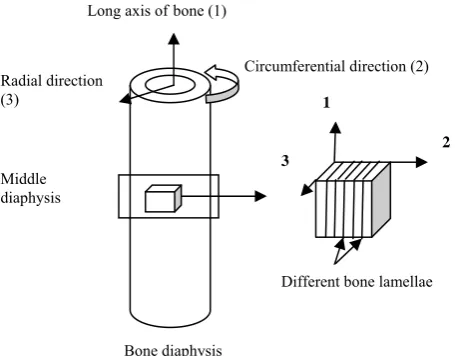
Fig. 1. Different material orientations of long bone employed in the present study.
direction was tested with the help of biaxial extensometer of gauge length 25 mm.
The shear properties of cortical bone were evaluated using Iosipescu shear test method. Four specimens were obtained from femoral mid diaphysis with dimensions 3 mm (thickness) x 20 mm (width) x 80 mm (length) and a 90° notch of length 4 mm was machined on each edge of the specimen at the mid length as per the ASTM standard [16]. In order to keep the specimens wet and to avoid heating during the various stages of tissue preparation a constant spray of saline solution was supplied. All specimens were stored at room temperature in a solution of 50% saline and 50% ethanol at all time until testing. The values of average shear stress (τ12), shear strain (γ12), longitudinal shear
modulus (G12) and transverse shear modulus (G23) were
calculated using appropriate equations as described in a previous study [17]. The orientations of bone samples used in this study are shown in Fig.1.
To obtain the apparent density of cortical bone rectangular samples were cut from the tested longitudinal and transverse tensile specimens using a diamond wheel (Isomet 4000). The volume of specimen was obtained after measuring its dimensions. The specimens were then hydrated overnight and the wet weight was recorded. The apparent density of the specimen was calculated by dividing wet weight to the volume of the specimen.
The anisotropic yield behavior of cortical bone was modeled through the use of yield stress ratios Rij. In this case
the yield ratios were defined with respect to a reference yield stress, σo (user-defined reference yield stress specified
for the material plasticity definition), such that if ( ) is applied as the only non zero stress, the corresponding yield stress is Rij.σo. For anisotropic yielding Hill’s potential
function can be expressed in terms of rectangular stress components as given in equation (1),
2 2 2 1
Where F, G, H, L, M and N are constants obtained from testings conducted in different orientations and defined as,
1 2
1 1 1
2
1 2
1 1 1
2
1 2
1 1 1
2
3
2 2 ,
3
2 2 and
3
2 2
Where Rij are the anisotropic yield stress ratios given as,
is the measured yield stress value when is applied as the only non zero stress component and /√3.
The flow rule can be described as,
, (4)
From the definition of f above,
2 2 2
(5)
Cortical bone is considered to be stronger and stiffer along the diaphysial axis (1) as compared to the transverse direction (2) whereas comparatively smaller differences in modulus and strength properties have been reported [18-21] between the radial (3) and circumferential directions (2). The bone material can therefore be considered as a transversely isotropic material for FE simulation.
The linear elastic material behavior for cortical bone was defined as;
(6) Where σ is the total stress (true stress), is the fourth-order elasticity tensor and is the total elastic strain (log strain). For 2-3 plane to be the plane of isotropy at every point, transverse isotropy requires that E1 = Et, E2 = E3 = Ep, ν12 = ν13 = νtp, ν21 = ν31 = νpt and G12 = G13 = Gt where p and
t stand for in-plane and transverse respectively. νtp and νpt
are not equal and are related by,
= , = , = , = , = ,
[image:2.595.47.275.278.456.2](a)
(b)
(c)
(a) (b)
(c)
(a) (b)
(c) (7)
The compliance matrix for transversely isotropic material reduces to;
1 0 0 0
1 0 0 0
1 0 0 0
1
0 0 0 0 0
1
0 0 0 0 0
1
0 0 0 0 0
p tp
p p t
p tp
p p t
pt pt
p p t
p
t
t
E E E
E E E
E E E
G
G
G
The FE simulation of uniaxial and biaxial tests on buffalo femoral cortical bone was carried out using the commercially available ABAQUS code. The uniaxial and biaxial specimens were modeled in three dimensional space as shown in Fig. 2.
[image:3.595.350.492.53.293.2]
Fig. 2. The three dimensional finite element models for (a) longitudinal tensile (b) transverse tensile and (c) biaxial specimens of cortical bone.
These models were discretized with second order 20-noded brick (hexahedra) elements. Gauss integration is almost always used with second order isoperimetric elements. The gauss points corresponding to reduced integration are the Barlow points at which the strains are most accurately predicted if the elements are well shaped. The uniaxial longitudinal and transverse models consist of 11020 (1998 elements) and 21940 (4566 elements) nodes respectively. The biaxial model consists of 4947 nodes and 900 elements. The FE models of different specimens along with the mesh are shown in Fig. 3.
[image:3.595.46.292.129.248.2]The local material orientations were defined for each model using the rectangular coordinate system as shown in Fig. 4. For all different models X axis was taken along the diaphysial (1) axis whereas Y and Z axis were considered along the circumferential (2) and radial (3) directions of the long bone.
[image:3.595.80.223.325.543.2]
Fig. 3. FE models of (a) uniaxial longitudinal (b) uniaxial transverse and (c) biaxial specimens of cortical bone along with mesh.
Fig. 4. Material orientations considered for (a) longitudinal tensile (b) transverse tensile and (c) biaxial models of cortical bone.
The FEM for the bone samples was employed using a mathematical model namely the incremental plasticity model, in which true stresses ( ) and true plastic strains ( ) were specified. The true stresses and true strains for cortical bone were determined from experimentally obtained nominal stresses ( ) and strains ( ) values using equations (9) and (10). The relationship between true stress and true plastic strain used in the simulation is given in equation (11).
1 (9)
ln 1 (10)
[image:3.595.332.515.344.589.2](a) (b)
0.00 0.01 0.02 0.03 0.04 0
40 80 120 160 200
Tru
e
S
tr
e
s
s
(
M
Pa)
True Strain Experimental FEM
(11)
Considering bone to be transversely isotropic material and using Hills criterion for anisotropic yielding, output results of the uniaxial longitudinal tensile model were analyzed first. After getting satisfactory results the same material properties were used to the uniaxial transverse tensile model of cortical bone by specifying different material orientations. The output results of FE model of uniaxial transverse tensile test were then compared with the experimental results for the validity of the approach and finally the biaxial FE modal of cortical bone was analyzed.
III. RESULTS AND DISCUSSION
The mechanical properties of buffalo femoral cortical bone such as elastic modulus (E1 and E2), shear modulus
(G12 and G23), yield strength in the case of longitudinal
tensile (σ1
yt), transverse tensile (σ2yt) and Iosipescu shear
testing (σ12
ys and σ23ys ), Poisson’s ratio (ν12 and ν23) and
apparent density (ρ1 and ρ2) obtained from different
experiments are listed in Table 1.
[image:4.595.322.518.100.269.2]The anisotropic yield ratios were determined for cortical bone considering yield stress for longitudinal direction as the reference yield stress (σo), and the same are listed in
Table 2.
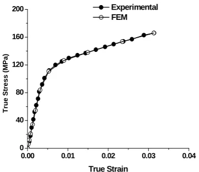
The true stress and true strain values for cortical bone in longitudinal direction were evaluated from experimental results as discussed earlier and compared with the corresponding values obtained from FE simulation. The comparison of true stress vs true strain curves obtained from the experimental testing and the FE simulation is shown in Fig. 5 whereas the corresponding contour profiles of Von-Mises and principal stresses are presented in Fig. 6.
The FE model of cortical bone in transverse direction (2)
[image:4.595.81.264.364.525.2]was further analyzed using the same material properties and yield criterion. The loading direction in this case was defined along the circumferential direction (2) of long bone.
Fig. 6. Contour profiles of (a) Von-Mises and (b) principal stresses for uniaxial longitudinal tensile test.
The comparison of true stress vs true strain curves obtained from experimental and FE modeling for transverse direction is shown in Fig. 7 and the contour profiles of Von-mises and principal stresses are shown in Fig 8.
TABLEI
PROPERTIES OF CORTICAL BONE ALONG DIFFERENT
MATERIAL ORIENTATIONS
Properties Units Values
E1 GPa 27.3
E2 GPa 17.1
G12 GPa 8.10
G23 GPa 5.77
σ1
yt MPa 81.6
σ2
yt MPa 61.9
σ12
ys MPa 51.2
σ23
ys MPa 41.3
ν12 --- 0.44
ν23 --- 0.48
ρ1 g/cm3 2.04
ρ2 g/cm3 1.96
The values reported here are the average values.
TABLE2
ANISOTROPIC YIELD STRESS RATIOS FOR BUFFALO FEMORAL
CORTICAL BONE
R11 R22 R33 R12 R13 R23
1 0.76 0.76 1.08 1.08 0.88
Fig. 5. Comparison of true stress-stain curves obtained from experimental testing and FE simulation of uniaxial longitudinal tensile test.
0.0000 0.0025 0.0050 0.0075 0.0100 0
20 40 60 80 100
Tr
ue
S
tr
e
s
s
(M
Pa)
True Strain Experimental FEM
[image:4.595.322.509.588.764.2]0.000 0.005 0.010 0.015 0.020 0
35 70 105 140
T
ru
e
St
re
s
s
(M
Pa
)
[image:5.595.64.278.55.204.2]True Strain Longitudinal direction Transverse direction
Fig. 8. Contour profiles of (a) Von-Mises and (b) principal stresses for uniaxial transverse tensile test.
[image:5.595.323.509.186.377.2]After getting satisfactory results from uniaxial model of cortical bone, the mechanical behavior of cortical bone under biaxial loading was analyzed using FE modeling. The contour profiles of Von-Mises and maximum principal stresses for biaxial model are shown in Fig. 9 whereas the same for in-plane ( ) and transverse ( ) shear stresses are shown in Fig. 10.
Fig. 9. Contour profiles of (a) Von-Mises and (b) principal stresses for biaxial model of cortical bone.
Ifyou are using Word, use either the Microsoft Equation
Fig. 10. Contour profiles of (a) in-plane and (b) transverse shear stresses for biaxial model of cortical bone.
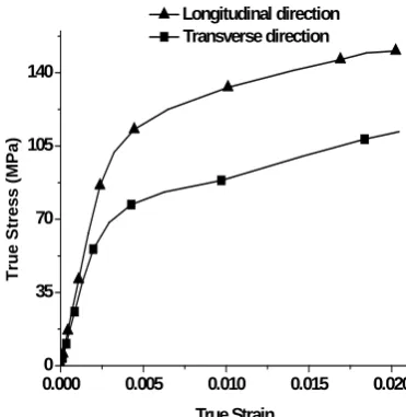
For biaxial model the behavior of stress - strain curves in both longitudinal and transverse directions was also analyzed. The comparison of stress-strain diagrams for two directions of loading is shown in Fig. 11. The nature of equivalent plastic strain vs Von-Mises stress curve for biaxial modeling is shown in Fig. 12.
It is evident from Fig. 5 that the stress-strain data obtained from FE model of uniaxial longitudinal tensile test shows good agreement with the experimental results. For uniaxial transverse tensile testing the stress-strain results
obtained from experiments and the FE modeling show almost similar behavior up to the yield point (corresponding to 0.002 strain offset point) and even beyond that up to a strain value of 0.006 as per Fig. 7. However the results of FE modeling start deviating from the experimental results as material hardening take place. The stress-strain curve of FE model shows higher hardening rate as compared to the experimental curve. This deviation may be due the assumption of constant yield ratios (corresponding to the initial yield point) for FE modeling.
Fig. 12. Equivalent plastic strain vs Von-Mises stress curve for biaxial model of cortical bone.
For the case of biaxial loading the Von-Mises and principal stress were observed to be higher along the longitudinal direction of cortical bone as shown in Fig. 9. The maximum values of in-plane and transverse shear stresses were noticed at the four corners of the specimen as per Fig. 10. This shows that failure in case of biaxial loading will initiate from the corners of the specimen as bone material is considered to be weaker in shear.
It was also noticed from the study that cortical bone has higher stiffness values in longitudinal and transverse directions for biaxial loading as compared to the uniaxial
(a) (b)
[image:5.595.48.287.349.459.2](a) (b)
Fig. 11. Compression of stress-strain diagrams for longitudinal and transverse directions of loading for biaxial model of cortical bone.
0.00 0.01 0.02 0.03
0 60 120
V
on-M
is
es S
tr
ess
(
M
P
a)
Equivalent Plastic Strain
[image:5.595.323.524.431.616.2] [image:5.595.50.289.509.618.2]loading. The values of longitudinal and transverse stiffness for biaxial loading were observed to be 1.4 and 1.8 times higher than the corresponding values for uniaxial loading. This shows an improved behavior of cortical bone under biaxial loading but experimental evidences are needed to justify this behavior.
The results show that the Hill’s criterion gives good results for FE modeling of cortical bone and can be used for multidirectional loading situations in bone mechanics to predict the fracture locations and to analyze the stress-strain behavior of anisotropic biological materials such as bone.
IV. CONCLUSION
The anisotropic behavior of cortical bone was modeled using Finite Element Modeling. Bone material was considered to be transversely isotropic in nature having five elastic constants. Anisotropic yielding in cortical bone was modeled using the Hill’s criterion. The longitudinal and transverse tensile models of cortical bone were found to be having good agreements with the experimental results. The FE modeling was further extended to biaxial loading in order to predict the behavior of cortical bone under multi-axial loading situation and improved behavior of cortical bone was observed under biaxial loading. The study shows that the Hills criterion gives better results for anisotropic yielding in bone material and can be effectively used for different combination of loading situations in case of complex biological materials.
REFERENCES
[1] S. Weiner, and H. D. Wagner, “The material bone: structure-mechanical function relations,” Ann Rev Mater Sci, vol. 28, pp. 271-298, 1998.
[2] R. A. Robinson, and S. R. Elliot, “The water content of bone: I. The mass of water inorganic crystals, organic matrix, and ‘CO2 space’ components in a unit volume of dog bone,” Journal of Bone Joint Surgery, vol. 39 A, pp. 167-188, 1957.
[3] R. B. Martin, Porosity and specific surface of bone. CRC Critical Reviews, 1984.
[4] E. Lucchinetti, “Composite models of bone properties,” in Bone Mechanics Handbook, 2nd ed. ch. 3, Boca Raton, Ed. FL: CRC Press, 2001, pp. 12.1–12.19.
[5] Z. Yosibash, N. Trabelsi, and C. Milgrom, “Reliable simulation of human proximal femur by higher-order finite element analysis validated by experimental observations,” Journal of Biomechanics, vol. 40, pp. 3688-3699, 2007.
[6] V. Baca, Z. Horak, P. Mikulenka, and V. Dzupa, “Comparison of an inhomogeneous orthotropic and isotropic material model used for FE analyses,” Medical Engineering & Physics, vol. 30, pp. 924-930, 2008.
[7] J. H. Keyak, and S. A. Rossi, “Prediction of femoral fracture load using finite element models: an examination of stress- and strain based failure theories,” Journal of Biomechanics, vol. 33, pp. 209-214, 2000.
[8] U. V. Pise, A. D. Bhatt, R. K. Srivastava, and R. Warkedkar, “A B-spline based heterogeneous modeling and analysis of proximal femur with graded element,” Journal of Biomechanics, vol. 42, pp. 1981-1988, 2009.
[9] W. R. Taylor, E. Roland, H. Ploeg, D. Hertig, R. Klabunde, M. D. Warner, M. C. Hobatho, L. Rakotomanana, and S. E. Clift, “Determination of orthotropic bone elstic constants using FEA and model analysis,” Journal of Biomechanics, vol. 35, pp. 767-773, 2002.
[10] J. H. Keyak, “Improved prediction of proximal femoral fracture load using nonlinear finite element models,” Medical Engineering & Physics, vol. 23, pp. 165-173, 2001.
[11] J. C. Lotz, E. J. Cheal, and W. C. Hayes, “Fracture predictionfor the proximal femur using finite element models: Part II-Nonlinear analysis,” Journal of Biomechanical Engineering, vol. 113, pp. 361-365, 1991.
[12] R. A. Simoes JA, “Tetrahedral versus hexahedral finite elements in numerical modeling of the proximal femur,” Medical Engineering & Physics, vol. 28, pp. 916-924, 2006.
[13] J. H. Keyak, and Y. Falkinstein, “Comparison of in situ and in vitro CT scans-based finite element model prediction of proximal femoral fracture load,” Medical Engineering & Physics, vol. 25, pp. 781-787, 2003.
[14] L. Peng, J. Bai, X. Zeng, and Y. Zhou, “Comparison of isotropic and orthotropic material property assignments on femoral finite element models under two loading conditions,” Medical Engineering & Physics, vol. 28, pp. 227-233, 2006.
[15] D. C. Wirtz, T. Pandorf, F. Portheine, K. Radermacher, N. Schiffers, A. Prescher, D. Weichert and F. U. Niethard, “Concept and development of an orthotropic FE model of the proximal femur,”
Journal of Biomechanics, vol. 36, pp. 289-293, 2003.
[16] Standard test method for shear properties of composite materials by the V-notched beam method, ASTM Standard: D5379 / D5379 M-98, 1998.
[17] N. K. Sharma, D. K. Sehgal, and R. K. Pandey, “Studies on locational variation of shear properties in cortical bone with Iosipescu shear test,” Applied Mechanics and Materials, vol. 148-149, pp. 276-281, 2012.
[18] R. B. Ashman, S. C. Cowin, W. C. Van Buskirk, and J. C. Rice, “A continuous wave technique for the measurement of the elastic properties of cortical bone,” Journal of Biomechanics, vol. 17, pp. 349-361, 1984.
[19] J. L. Katz, and A. Meunier, “The elastic anisotropy of bone,” Journal of Biomechanics, vol. 20, pp. 1063-1070, 1987.
[20] D. T. Reilly, and A. H. Burstein, “The mechanical properties of cortical bone,” Journal of Bone Joint Surgery, vol. 56A, pp. 1001-1022, 1974.
[21] X. N. Dong, and X. E. Guo, “The dependence of transversely isotropic elasticity of human femoral cortical bone on porosity,”