Accuracy of Structure from Motion models in comparison with terrestrial laser scanner for the analysis of DBH and height influence on error behaviour

JOURNAL OF FOREST SCIENCE, 62, 2016 (8): 357–365 doi: 10.17221/92/2015-JFS

Accuracy of Structure from Motion models in comparison

with terrestrial laser scanner for the analysis of DBH and

height influence on error behaviour

D. Panagiotidis, P. Surový, K. Kuželka

Department of Forest Management, Faculty of Forestry and Wood Sciences, Czech University of Life Sciences Prague, Prague, Czech Republic

ABSTRACT: With the advantage of Structure from Motion technique, we reconstructed three-dimensional structures

from two-dimensional image sequences in a circular plot with a radius of 6 m. The main objective of this research was to clarify the potential of using a low cost hand-held camera for evaluation of the stem accuracy reconstruc-tion, through the comparison of data from two different point clouds. The first cloud comprises data collected with a digital camera that are compared with those collected by direct measurement of the FARO® _{Focus3D S120 laser}

scanner. Photos were taken in a circular plot of pine trees using the stop-and-go method. We estimated the Euclidean distance for corresponding points for both clouds and we found out that most of the points with error less than 11 cm are concentrated mainly on the ground. Regression analysis showed a significant relationship between height above ground and error, the error is more pronounced for points located higher on the stems. As expected, no dependence was found between the error of the points and the diameter at breast height of their respective stems.

Keywords: hand-held digital camera; point cloud; stem optimization; image segmentation; photogrammetry

Supported by the Czech University of Life Sciences Prague, Project No. B07/15, and by the Ministry of Agriculture of the Czech Republic, Project No. QJ1520187.

An imaging system was developed by Juujärvi et al. (1998) in order to automate the study of tree mea-surement characteristics by using terrestrial im-ages. This system consisted of three main parts: (i) calibrated camera, (ii) laser distance measurement device, (iii) calibration stick. The stem curvature of Scots pines was estimated using the principle (of taper model) for the image interpretation. Accord-ing to a research study by Melkas et al. (2008), the laser camera development integrated a digital cam-era and a laser line gencam-erator to measure diameter at breast height (DBH) of individual trees. Results of the automated diameter measurement detected 57.4% of valid observations. The standard devia-tion of the measurable observadevia-tions was 1.27 cm. A 360° panorama plot image was used by Dick et al. (2010) to produce a stem map. Higher point densities, which can be produced with a terrestrial laser scanner (TLS), can fill the gap between laser

is decreasing amplitude of the coverage area with increasing distance to the sensor (in case that the scanner is of low quality). The other focuses on the inability of the laser pulses to penetrate through occluding vegetation, which results in insufficient laser point density and in turn leads to underesti-mations compared to manually collected field data (Van der Zande et al. 2006; Moskal, Zheng 2012). The use of dual-wavelength TLS provides a clear separation between leaf returns, returns from branches, ground and returns from the stems. We can distinguish three categories of field measure-ments. The first approach is a single-scan approach when the laser scanner is placed at the centre of the plot and one full 360° scan in horizontal axes and a 310° scan are made. The low detection rate is a major drawback of this method, since not all trees are scanned due to the occlusion effects. The second approach is a multi-scan approach. In this method the laser scanner is placed in various posi-tions inside and outside of the plot. Consequently, this method provides better quality of data as the produced point clouds are based on merged point cloud records of trees taken from different posi-tions. Finally, there is a multi-single-scan when several point clouds are processed individually and data sets are merged at the level of features (Brol-ly, Kiraly 2009; Murphy et al. 2010; Lovell et al. 2011; Liang et al. 2012). Nowadays, with the use of multi-view stereopsis (MVS) techniques, combin-ing computer vision and photogrammetry (Furu-kawa, Ponce 2007), and by using algorithms like: SIFT introduced by Lowe (2004) and SURF by Bay et al. (2008), it is possible to use common optical cameras for the reconstruction of 3D objects in or-der to improve the representation of tree stem and crown structure. One of the advantages when us-ing a hand-held camera is the ability to regulate the amount of shots to fully cover a tree structure in terms of elevation. However, according to Surový et al. (2016), when they tried to examine the trend between height, azimuth and the error of recon-struction, there was a higher error in the areas of lower visibility (upper and lower parts of the stem). Point cloud generation based on MVS and image matching can fill gaps that are produced by TLS. The former has been proven thought by the recent studies (Dandois, Elis 2010; Lucieer et al. 2011; Neitzel, Klonowski 2011; Rosnell, Honka-vaara 2012), where they have successfully adopted MVS to derive a dense point cloud from optical im-ages in a complex terrain with a precision of 1–2 cm point spacing. However, the real accuracy of each method is uncertain since it is of high

correla-tion and effectiveness by a series of other mainly in-situ forest parameters. The latest technological improvements and recent discoveries in construc-tion of 3D modelling of a forest structure propose to evaluate the accuracy of the models by using a reference model (usually the one with the highest precision).

The goal of this study was to clarify the creation of photo-reconstructed models of tree stems through comparison with TLS data, by evaluating the error distribution in terms of two independent variables (height and DBH). This was done in order to clarify whether or not a low cost hand-held camera can be used effectively for stem accuracy reconstruction. For examining the behaviour and reliability of each method, Akca et al. (2010) suggested internal ac-curacy assessment of a 3D model by bringing the whole xyz surface in correspondence, by using the Euclidean distance and least squares method be-tween the two point cloud surfaces.

MATERIAL AND METHODS

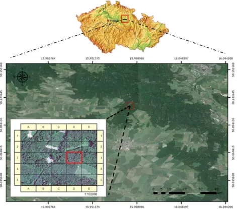
Study area. The district area Plchůvky in the Czech Republic belongs to the state forests, under the Choceň Forest Administration, and is located in the eastern part of the town of Pardubice (Fig. 1). It extends geographically from 50°02'15.7661''N to 16°08'29.5501''E, with an altitude of 290 m a.s.l. The research plot is within an area of mainly acidic de-position. The plot also consisted of coniferous trees and specifically of Pinus sylvestris Linnaeus, with average tree height of 12 m and average diameter of 20 cm. The research plot was circular, with 6 m radius, on a flat field without slope.

Laser scanner. Terrestrial laser scanner data was acquired in April 2015 by using a FARO® _Focus3D

S120 laser scanner (FARO®_{, Lake Mary, USA). The}

scanner is a small, light and fully portable device able to provide distance accuracy up to ± 2 mm and range from 0.6 up to 130 m. To calibrate the laser scanner we used the field instant method, while for the identification of co-registration, for the scan registration we chose the use of six spheres for elaborating better performance. The procedure of referencing, orientation and filtering of our data in the scans is a necessary procedure for remov-ing all the isolated points, by usremov-ing the SCENE 3D laser scanner software (Version 5.0, 2015). The SCENE software is laser scanning software specifi-cally designed for the FARO® _{Focus3D processing}

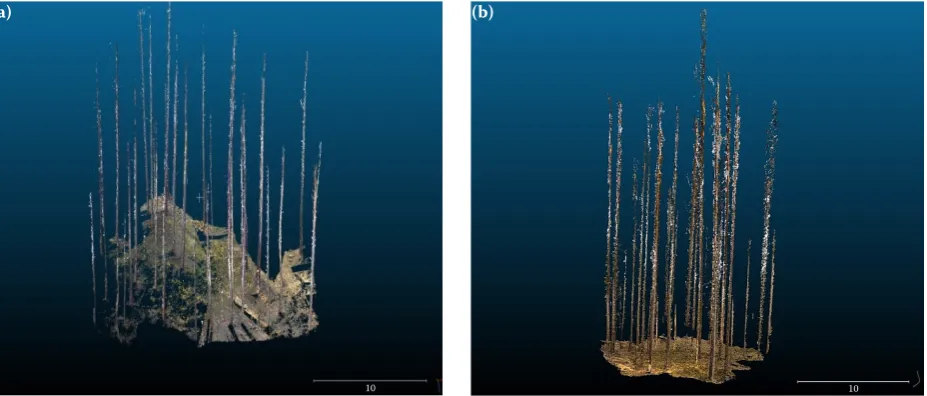
registra-tion and posiregistra-tioning. In addiregistra-tion, to collect data on a tree level, we used the multi-scan approach. The laser scanner is initially placed at the centre of the circular plot, then one full field-of-view scan (e.g. 360° in horizontal direction and 310° in verti-cal direction) is made, producing a 3D model of the research plot (Fig. 2a, in this phase the model is af-ter the removal of branches). Moreover, we took six additional scans, which were made in different di-rections around the borders of the plot in order to increase the point cloud accuracy of the tree stems.

Image acquisition description. Image data was taken on the same day as the TLS. For the image acquisition a Nikon 1 V1 hand-held digital camera (Nikon, Tokyo, Japan) with focal length of 10 mm and 10.1 million of effective pixels was used. We set the operational parameters to ISO sensitivity 200, exposure time 0.01 s and aperture 3.6. By using the stop-and-go method and by following the photo-graphic path (perimeter of the circular plot), we

collected in total 350 photos regularly distributed around the stems. That means that the operator stood still while taking a photo and then moved to the next position by taking a small step aside. Every time we changed the position, we made a small step to ensure that the covering angle and to-tal amount of pictures were adequate for best per-formance alignment during processing in Agisoft PhotoScan©_{software (Version 1.2.2, 2015) and}

alignment, as well as the reconstruction of sparse/ dense point cloud afterwards, was done using an automatic camera calibration setup, by means of the Agisoft PhotoScan© _{software. In the image}

re-construction process using Structure from Motion Technique, 318 out of the original set of 350 im-ages were finally aligned, the left 32 imim-ages were automatically excluded from the processing due to poor quality. The mesh was reconstructed from the dense field, while for the texture construction in Agisoft PhotoScan© _{software we used a density}

value of 4,096 × 2 in order to achieve a greater reso-lution of the final texture, producing a 3D model structure (Fig. 2b, the model in this phase like for the case of TLS above is also after the removal of branches). The reference points were then identi-fied on the texture model and the real world posi-tions from measurements were attributed to them. Software and statistics for data comparison. For the visualization of our data we used mainly two types of software: (i) Agisoft PhotoScan© _{for the}

construction and alignment of a point cloud from photographs, (ii) CloudCompare (Version 2.6.1, 2015) for the construction of a point cloud from TLS data. The latter is the open source software written in C++ for 3D point cloud and mesh pro-cessing, its power lies in the ability not only to visu-alize but also to compare point clouds representing the same object, received from different types of methods e.g. TLS and digital camera. Our method-ology for this research is based on an individual tree detection approach. Initially, before merging the two point clouds, we scaled the point cloud which was derived from photo-camera by using plastic points as reference points, with known dimensions (length and width), afterwards we proceeded to the

merged and aligned data with the two point clouds, which were taken with two different types of sen-sors: (i) photo images, (ii) laser scanner. At the end we visualized them in 3D space. More specifically, we aligned the two datasets by the method of pick-ing four equivalent point pairs. For mergpick-ing both point clouds, we used all of four selected point pairs at the bottom of the stems (intersected with ground points). Then, we proceeded to the com-parison of both point clouds and for the distance computation we used the CloudCompare software, with the cloud-cloud distance approach (distance between the two point clouds is the nearest neigh-bour distance, by using a kind of Hausdorff36 dis-tance algorithm for each point of the compared cloud). CloudCompare searches the nearest point in the reference cloud (TLS). This cloud should have the widest extents and the highest density and computes their Euclidean distance. At the second step, with the use of image segmentation and lo-cal statistilo-cal test tools, we could segment/filter a point cloud based on the local statistical behaviour of the active scalar field. If for example the active scalar field corresponds to distances and we know the distribution of the measurement noise, then we are able to filter the points for which the local sca-lar values seem to fit to the noise distribution. This allows us to ignore the outsiders and focus on the points with distances clearly out of the noise dis-tribution and to minimize the error caused by the branches and leaves. We also used the octree tool, which mainly resamples a cloud by replacing all the points inside each cell of the octree (at a given level of subdivision) by their centre of gravity. The level of subdivision at which the process is applied is chosen to roughly match the expected number of Fig. 2. Terrestrial laser scanner (a), digital camera (b) 3D model, both models after the image segmentation in RGB colours

(a) (b)

output points. Therefore, we used a default value of 8 for this study (Mémoli, Sapiro 2004). For the registration of matching models, we used picking point pairs in order to match the two clouds with the lowest possible error. Finally, we evaluated the probability density function for the non-reference model (data from the photo camera) by using the continuous Weibull probability distribution. It is the shape flexibility function which is able to fit to any type of data. The density function has the gen-eral form shown below (Eq. 1):

(1)

where:

x – location parameter,

a – scale parameter (x ≥ a, b > 0),

b – Weibull distribution shape parameter (x ≥ a, b > 0).

After that, we used again the segmentation tool, this time to cut the point cloud into smaller parts separated by a minimum distance. This approach allowed us to split the forest stand and extract in-dividual stems for better visualization and analysis. Detection of ground points and computation of height above ground for all points represent-ing stems were carried out usrepresent-ing LAStools (Ver-sion 141017, 2014). For data processing MATLAB R2012b (Version 8.0, 2012) with the Statistics and Machine Learning Toolbox was used. Linear re-gression between height above ground and Euclid-ian distance between point clouds was computed and its significance was tested. To determine DBH of the stems, points of above-ground height between 1.25 and 1.35 m were selected and

pro-jected onto a horizontal plane. Cluster analysis was applied to the resulting two-dimensional data and corresponding points were segmented into parts for surfaces of individual stems. For each segment, an ellipse was fitted to the data points representing the perimeter at breast height. For ellipse fitting, we used the algorithm proposed by Fitzgibbon et al. (1999). The major axis of the el-lipses was considered to be the average diameters of the stems.

RESULTS

Results of alignment comparison

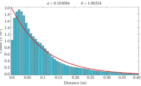
We divided the results into two categories. The first category includes both clouds and aligns them. The alignment resulted in a root mean square error of 0.11 m and the second category concerned the analy-sis of DBH and height influence on error behaviour. The total number of points after the segmentation of image from branches, leaves and outlier values was 3,000,323 points (laser scanner). In this first category for comparison of alignment we involved points from all model meaning (ground and stems). The full range of matching points that was analysed ranges signifi-cantly between 0 and 0.11 m. However, from the his-togram (Fig. 3), the error is distributed with an interval range of 0–0.4 m (because the error tendency appears to be smoothly decreasing after 0.4 m according to our analysis and therefore we concluded that it is not necessary to be visualized in the graph for practical reasons). Fig. 3 also illustrates the Weibull distribu-tion shape parameter b = 1.00354, which represents the steepness of the slope of the curve for these spe-cific taxonomic values. The reverse “J” shape curve of the probability density function of Weibull distribu-tion, which was fitted to our data, indicates that the error between the points of the two clouds is less or equal than 11 cm. The latter is a filtering process by which the outliers are excluded before any statistical calculation, in order to avoid biased texture develop-ment mainly focused on the stems. Fig. 4a clarifies that most of the points with error less than 11 cm in distance are on the ground, while for the stems errors are greater than 11 cm.

Error behaviour between height and DBH

In this part, we tried to evaluate the error dis-tribution in terms of two independent variables: (i) height, (ii) DBH. For both variables we seg-Fig. 3. Distribution of values from the alignment of both point

clouds (laser scanner and digital camera), x-axis – absolute distance in meters for all points between the two clouds (laser scanner and digital camera), y-axis – total amount of counted points from both point clouds

a – scale parameter, b – Weibull distribution shape parameter

a = 0.103084 b = 1.00354

0.0 0.05 0.1 0.15 0.20 0.25 0.30 0.35 0.40 Distance (m)

2.0 1.8 1.6 1.4 1.2 1.0 0.8 0.6 0.4 0.2 0.0

Coun

t (× 10

5)

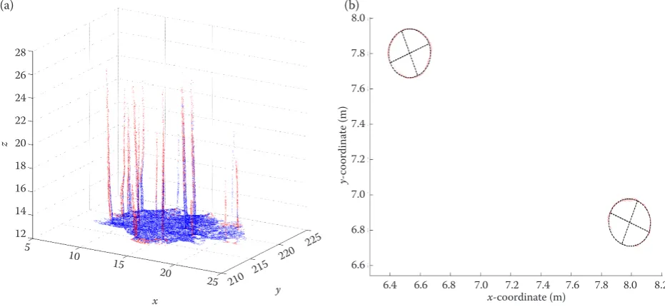
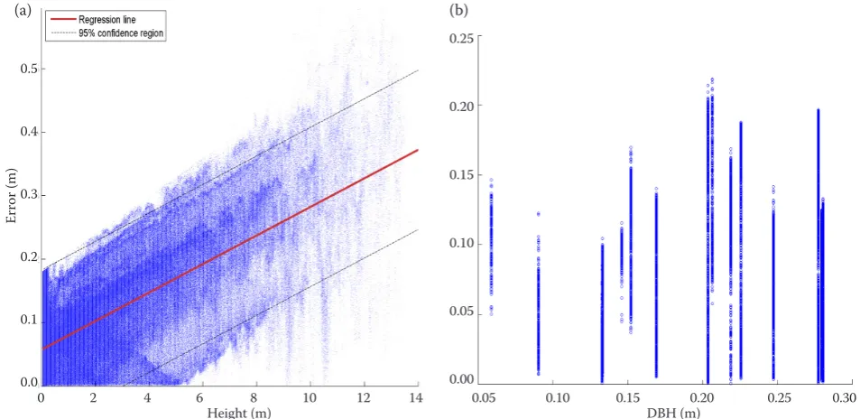
mented and isolated only the tree stems, so to be able to examine and analyse the distribution of error in terms of height and DBH. The amount of point reduction in this phase was almost 96%. The total number of trees involved in the research plot (isolated for further evaluation) was n = 15. Fig. 5a shows the result from the regression analysis be-tween the correlations of height and error, which showed that the error tends to increase linearly as the height of the trees increases, more specifically at the upper part of the stem, where we have areas of lower visibility. Statistical values of the regres-sion line for height-error relationship are shown in Table 1. Fig. 4b displays the points representing the stem surface at the height of 1.3 m and ellipses fitted to these points. This serves to determine the DBH of the individual trees. Fig. 5b shows the relation of DBH of individual trees inside the plot and the error of respective points belonging to the stems. In Fig. 5b, by using a multivariate technique so called Principal Components Analysis (PCA), each column with blue colour representing one stem, where on the x-axis we have the diameter of each stem at breast height and on the vertical y-axis the distribution of error for different diameter values. It is obvious that the error is not dependent on the DBH of the trees, forming a non-linear behaviour.

DISCUSSION AND CONCLUSIONS

The recent advances in computer vision enable the potential of terrain surface reconstruction from remotely sensed images Lucieer et al. (2011) and therefore can be used for 3D stem reconstruction. In fact this method has a great potential, when com-pared to the laser scanner method. As demonstrated in this study, we introduced a method for point cloud comparison and processing by Agisoft PhotoScan©_,

CloudCompare and MATLAB software and we con-sider the information provided by the TLS as ground truth data due to: (i) higher precision, (ii) ability to create more points from fewer positions and conse-quently to increase the quality of the data. We manage to fit the two different point clouds, taken with differ-ent kind of sensors. In our study, both clouds were aligned by the equivalent point pair method, where we were able to determine identical trees in both clouds, only with the help of identical shapes and that is why because the models were not transformed to the same global coordinate system. In their research, Harwin and Lucieer (2012) used differential GPS technology in order to verify the level of accuracy of point clouds which were derived from photos. What they found was a clearly reconstructed terrain with an accuracy of around 2.5–4 cm.

Table 1. Statistical values of the regression line for height-error relationship

Error Coefficient R2 _{df Adjusted R}2 _RMSE

P1 × h + P2 P_P1 = 0.00225_{2 = 0.05773} 0.52 112.516 0.52 0.064

h – height, RMSE – root mean square error

Fig. 4. 3D point cloud (a), the points at a sample of two stems representing the cross-sectional cut at 1.3 m and their ellipsoid fit-ting (b); the colour indicates the value of the error, blue points have the error lower than 0.1 m, the error of red points was higher (a) (b)

28 26 24 22 20 18 16 14 12

z

5 10 15 20 25

210 215 220 225

x y

8.0

7.8

7.6

7.4

7.2

7.0

6.8

6.6

6.4 6.6 6.8 7.0 7.2 7.4 7.6 7.8 8.0 8.2

x-coordinate (m)

y

-c

oor

dina

Particularly, in this work we wanted to initially show if there were any significant differences in terms of data acquisition, acquired by two differ-ent methods (point cloud generation from TLS and photo images) and if such differences did exist, then we tried to approximate those differences with the help of some statistical analyses by using regression models. Our results from the first part of alignment comparison primarily verified the asymmetry of the data (by expressing a reverse “J” shape) in terms of distance between points. However, by looking on Fig. 4a, we clearly saw that most of the points with error less than 11 cm were concentrated mainly on the ground of the reconstructed model. Based on the above, accuracy was not similar at the part of the stems for both point clouds. Also, according to Surový et al. (2016), the fewer matching points on the stems from the same image indicate partially the inability of the photo camera to reconstruct more points especially at the higher parts of the tree stem and that is why error mostly greater than 11 cm was concentrated on tree stems and not on the points near and on the ground. Moreover, based on the histogram of Fig. 3, the modus of the deviations between the two point clouds was around 3 cm, clarifying that most appearing values of the point clouds were of higher accuracy and concertation on the ground compared to above-ground points. Secondly, we wanted to test the precision of point clouds by testing the two most common indepen-dent variables: DBH and height influence on error behaviour. More specifically, in this part we tried to evaluate the behaviour of error in terms of height

with respect to the incomplete tree stem structure derived from the point cloud, using camera photos. The detection rate evaluated and illustrated the de-crease of matching between the two point clouds, in regard to increasing height, forming a linear behav-iour. In their work, Fritz et al. (2013) used a simi-lar approach, except they used an unmanned aerial vehicle platform instead, mounted with an optical sensor instead of a hand-held camera and com-pared that data with TLS (FARO® _{Focus3D S120}

laser scanner). They came to the same conclusion, namely with the decrease of point matching with increasing height. This correlation of reconstruc-tion along the height axis, specifically in the case of data derived with the digital camera, is likely influ-enced by the density of the crown structure, fewer points and the long distance from the sensor and therefore it is considered to be parts of lower visi-bility. According to the results of the statistical met-rics analysis, the stem reconstruction at lower parts tends to become more accurate when examining the height distribution in correlation with the error behaviour at different height positions, while at a higher portion of the tree stem accuracy decreases and that could be the case of reduced ground sam-pling distance. An explanation which can be given is that the higher we go, the larger the deviation was because images taken from higher portions of the stem have a lower overlapping potential, therefore the shapes were not so clear and sharp as next to the ground. Regarding the dependence between the DBH of a tree and points of error belonging to the tree, there is no reason to suppose any such de-Fig. 5. Behaviour of error in terms of height – regression analysis (a), DBH – Principal Components Analysis (b)

(a) (b)

0.5

0.4

0.3

0.2

0.1

0.0

Er

ror (m)

0.25

0.20

0.15

0.10

0.05

0.00

0.05 0.10 0.15 0.20 0.25 0.30 DBH (m)

pendence. We preferred to use the PCA method, generally because of the simplification of data pro-cessing and analysis. The position of a point cannot be less or more precise according to the size of the object which it belongs to. Neither the visibility of the stem nor the reflectance and structure deter-mining the accuracy of points in the point cloud are affected by the DBH of the tree, there is a non-linear behaviour. All 15 stems, evaluated for DBH influence on error behaviour had approximately the same characteristics, meaning that most of the stems appeared to increase homogeneity (by hav-ing more or less the same or similar characteristics such as height and diameter distribution). This ex-pectation was also verified by our analysis. No such dependence was detected in the data.

References

Akca D., Freeman M., Sargent I., Gruen A. (2010): Quality assessment of 3D building data. The Photogrammetric Record, 25: 339–355.

Bay H., Ess A., Tuytelaars T., Van Gool L. (2008): Speeded Up Robust Features (SURF). Computer Vision and Image Understanding, 110: 346–359.

Brolly G., Kiraly G. (2009): Algorithms for stem mapping by means of terrestrial laser scanning. Acta Silvatica & Lignaria Hungarica, 5: 119–130.

Dandois J.P., Elis E.C. (2010): Remote sensing of vegeta-tion structure using computer vision. Remote Sensing, 2: 1157–1176.

Dassot M., Constant T., Fournier M. (2011): The use of ter-restrial LiDAR technology in forest science: Application fields, benefits and challenges. Annals of Forest Science, 68: 959–974.

Dick A.R., Kershaw J.A., MacLean D.A. (2010): Spatial tree mapping using photography. Northern Journal of Applied Forestry, 27: 68–74.

Fitzgibbon A., Pilu M., Fisher R.B. (1999): Direct least square fitting of ellipses. IEEE Transactions on Pattern Analysis and Machine Intelligence, 21: 476–480.

Fritz A., Kattenborn T., Koch B. (2013): UAV-based pho-togrammetric point clouds – tree stem mapping in open stands in comparison to terrestrial laser scanner point clouds. International Archives of the Photogrammetry, Remote Sensing and Spatial Information Sciences, XL-1/ W2: 141–146.

Furukawa Y., Ponce J. (2007): Accurate, dense and robust multi-view stereopsis. In: Proceedings of the 2007 IEEE Conference on Computer Vision and Pattern Recognition, Mineapolis, June 18–23, 2007: 1–8.

Harwin S., Lucieer A. (2012): Assessing the accuracy of geo-referenced point clouds produced via multi-view stereopsis

from unmanned aerial vehicle (UAV) imagery. Remote Sensing, 6: 1573–1599.

Hopkinson C., Chasmer L., Young Pow C., Treitz P. (2004): Assessing forest metrics with ground-based scanning Li-DAR. Canadian Journal of Forest Research, 34: 573–583. Huang H., Li Z., Gong P., Cheng X., Clinton N., Cao C., Ni

W., Wang L. (2011): Automated methods for measuring DBH and tree heights with a commercial scanning LiDAR. Photogrammetric Engineering and Remote Sensing, 77: 219–227.

Juujärvi J., Heikkonen J., Brandt S.S., Lampinen J. (1998): Digital image based tree measurement for forest inven-tory. In: Casasent D.P. (ed.): Proceedings of the 17th _SPIE

Conference on Intelligent Robots and Computer Vision: Algorithms, Techniques, and Active Vision, Boston, Oct 6, 1998: 114–123.

Lovell J.L., Jupp D.L.B., Newnham G.J., Culvenor D.S. (2011): Measuring tree stem diameters using intensity profiles from ground-based scanning LiDAR from a fixed viewpoint. ISPRS Journal Photogrammetry and Remote Sensing, 66: 46–55.

Lowe D.G. (2004): Method and apparatus for identifying scale invariant features in an image and use of same for locating an object in an image. US Patent 6,711,293. Mar 23, 2004. Liang X., Kankare V., Yu X., Hyyppa J., Holopainen M. (2014):

Automated stem curve measurement using terrestrial laser scanning. IEEE Transactions on Geoscience and Remote Sensing, 52: 1739–1748.

Liang X., Litkey P., Hyyppa J., Kaartinen H., Vastaranta M., Holopainen M. (2012): Automatic stem mapping using single-scan terrestrial laser scanning. IEEE Transactions on Geoscience and Remote Sensing, 50: 661–670. Lucieer A., Robinson S., Turner D. (2011): Unmanned aerial

vehicle (UAV) remote sensing for hyperspatial terrain mapping of Antarctic moss beds based on structure from motion (SfM) point clouds. In: Proceedings of the 34th

International Symposium on Remote Sensing of Environ-ment, Sydney, Apr 10–15, 2011: 11–15.

Maas H.G., Bienert A., Scheller S., Keane E. (2008): Automatic forest inventory parameter determination from terrestrial laser scanner data. International Journal of Remote Sens-ing, 29: 1579–1593.

Melkas T., Vastaranta M., Holopainen M. (2008): Accuracy and efficiency of the laser-camera. In: Hill R., Rosette J., Suárez J. (eds): Proceedings of SilviLaser 2008: 8th _{International}

Conference on LiDAR Applications in Forest Assessment and Inventory, Edinburgh, Sept 17–19, 2008: 315–324. Mémoli F., Sapiro G. (2004): Comparing point clouds.

In: Proceedings of the Eurographics/ACM SIGGRAPH Symposium on Geometry Processing, Nice, July 8–10, 2004: 32–40.

Murphy G.E., Acuna M.A., Dumbrell I. (2010): Tree value and log product yield determination in radiata pine (Pinus

ra-diata) plantations in Australia: Comparisons of terrestrial

laser scanning with a forest inventory system and manual measurements. Canadian Journal of Forest Research, 40: 2223–2233.

Neitzel F., Klonowski J. (2011): Mobile 3D mapping with a low-cost UAV system. International Archives of the Pho-togrammetry, Remote Sensing and Spatial Information Sciences, XXXVIII-1/C22: 1–6.

Rosnell T., Honkavaara E. (2012): Point cloud generation from aerial image data acquired by a quadcopter type micro unmanned aerial vehicle and a digital still camera. Sensors, 12: 453–480.

Strahler A.H., Jupp D.L.B., Woodcock C.E., Schaaf C.B., Yao T., Zhao F., Yang X., Lovell J., Culvenor D., Newnham G. (2008): Retrieval of forest structural parameters using a ground-based LiDAR instrument (Echidna®_{). Canadian}

Journal of Remote Sensing, 34: 426–440.

Surový P., Yoshimoto A., Panagiotidis D. (2016): Accuracy of reconstruction of the tree stem surface using terrestrial close-range photogrammetry. Remote Sensing, 8: 123. Van der Zande D., Hoet W., Jonckheere I., van Aardt J., Coppin P.

(2006): Influence of measurement set-up of ground-based LiDAR for derivation of tree structure. Agricultural and Forest Meteorology, 141: 147–160.

Received for publication October 12, 2015 Accepted after corrections July 19, 2016

Corresponding author:

Ing. Dimitrios Panagiotidis, Czech University of Life Sciences Prague, Faculty of Forestry and Wood Sciences, Department of Forest Management, Kamýcká 1176, 165 21 Prague 6-Suchdol, Czech Republic;