JOURNAL OF FOREST SCIENCE, 51, 2005 (10): 431–445
Tree growth models are implemented in forestry and ecology. They provide the advantage of an in-dividual tree modeling approach. Flexible reactions to very complicated phenomena are possible, for example, the relationship between tree mortality and competition. If we want to implement these models into current forestry practice as a tool for decision support, we must integrate thinning algorithms into the models. Automatic selection of thinning trees by specification of thinning concept, thinning amount, and thinning interval is assumption for an execu-tion of different thinning strategies and selecexecu-tion of optimal one. A lot of models exist in Europe (SILVA, BWIN, PROGNAUS, MOSES, STAND, DRYMOS, CORKFITS) and each of them includes some thin-ning tool. Thinthin-ning concepts are modeled by differ-ent approaches. Some models use algorithms based on empirical data analysis, for example, the logistic model by LEDERMANN (2002). Several models are es-tablished in an analytical way, for example, the fuzzy model by KAHN (1995). Other models are based on knowledge and heuristic principles, for example, the expert system ThiCon (DAUME, ROBERTSON 2000). The models can be deterministic or stochastic.
The model SIBYLA (FABRIKA 2003a) was devel-oped during the period 2001–2004. The development has been supported by the Europe Committee as a
part of the 5th Framework Program of the European
Union. The model is built on SILVA modeling prin-ciples (PRETZSCH 2001). An new software solution has been created. The growth simulator SILVA 2.2 includes a comprehensive tool for thinning concepts (KAHN 1995), but this tool is not direct applicable to Slovakian conditions. The thinning model of SILVA 2.2 does not consider tree quality. Tree quality is usually estimated in Slovakian forest inventories and seems to be very important. Also, some specific thinning concepts are not included in the SILVA 2.2 model. Therefore, we have decided to develop our own thinning engine. The thinning engine is built from a combination of new algorithms and existing algorithms and approaches (ASSMANN 1961; HALAJ 1985; HALAJ et al. 1986; JOHANN 1982; KAHN 1995; KONŠEL 1931; KORPEĽ et al. 1991; LIOCURT 1898; MEYER 1952; PRETZSCH 2001; REMIŠ et al. 1988; REYNOLDS 1999; SCHÄDELIN 1942; ŠTEFANČÍK 1974, 1977, 1984). The model is created in an analytical way and some parts of it are tested on experimental
Algorithms and software solution of thinning models
for SIBYLA growth simulator
M. FABRIKA, J. ĎURSKÝ
Faculty of Forestry, Department of Forest Management and Geodesy,
Technical University in Zvolen, Zvolen, Slovak Republic
ABSTRACT: The paper deals with a proposal for a thinning model for the growth simulator SIBYLA. The model is based on an analytical-causal modeling approach. Some partial theorems are tested on experimental data from thinning sample plots. The model is composed of the following components: the model of bio-sociological tree status, the model for score of existence, the model for type of selection, the model for amount of thinning, and the aggregated model of the thinning concept. The appropriate combination of type and amount of thinning allows the user to perform the following thinning concepts: thinning from below, thinning from above, neutral thinning, crop tree thinning, target diameter thinning, target frequency (equilibrium) curve thinning, clear cutting, and thinning by list (interactive thin-ning). A software solution of the algorithms, and an example of different thinning concepts for selected forest stands is presented at the end of the paper along with a discussion about the advantages and disadvantages of the thinning model compared to the SILVA 2.2 model.
data set. Experimental data comes from thinning experiments of the Department of Forest Manage-ment and Geodesy in Zvolen and the Forest Research Institute in Zvolen. The model is composed from the following components: a model of bio-sociological tree status, a model for score of existence, a model for type of selection, a model for amount of thinning and an aggregated model of the thinning concept. This paper presents algorithms of the thinning models. The model has been developed in frame of individual research by the authors and has been co-supported by foundation of ALEXANDER VON HUMBOLDT in the years 2004–2005.
METHODOLOGY
Model of bio-sociological tree status
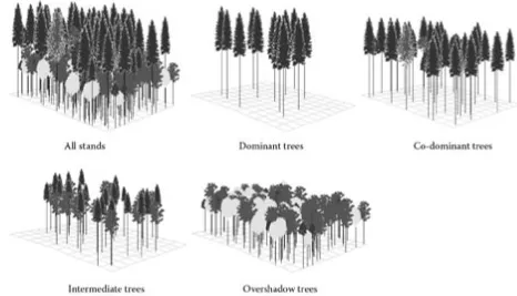
Bio-sociological tree status plays an important role in some thinning concepts, for example, for selec-tion of thinning trees in thinning from below and thinning from above or for selection of crop trees. A simplified classification scale by KONŠEL (1931) has been used:
1 – dominant trees, 2 – co-dominant trees, 3 – intermediate trees, 4 – overshadow trees.
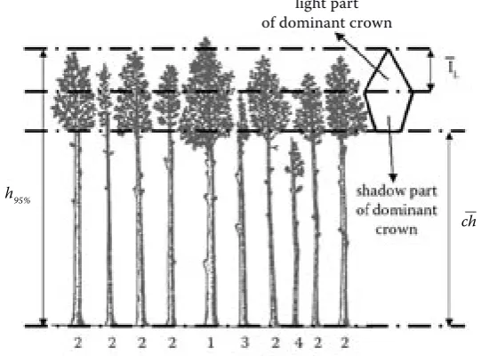
Classification algorithms (BIOSOC model, Fig. 1) are based on tree heights and modeling of tree crown parameters. First, the dominant height of the plot
(h95%) is calculated. The dominant height is the limit
between dominant and co-dominant trees. Utiliza-tion of dominant height has arisen by investigaUtiliza-tion on thinning research plots. Then, the height to the base
of the crown (ch) and the length of the light part of the
crown (lL) are calculated for the dominant height by
k m d ij2 . hij
Σ Σ[(
––––––)
. ch (95%)i]
i=1 j=1 100ch = ––––––––––––––––––– (1)
k m
d ij2 . hij
Σ Σ (
–––––)
i=1 j=1 100
k m
dij2 . h ij
Σ Σ[(
––––––)
. lL (95%)i]
i=1 j=1 100lL = ––––––––––––––––––– (2)
k m
d ij2 . hij
Σ Σ (
–––––)
i=1 j=1 100
where: dij, hij – diameters and heights of trees,
k – number of tree species,
m – number of trees for corresponding tree species,
ch(95%)i, lL(95%)i – height to the base of the crown and length of light part of the crown for trees of dominant height.
The heights to the base of the crown and lengths of the light part of the crown are calculated by PRETZSCH (2001). The classification of the trees into scale is performed by the rule
hi ≥ h95% 1
(hi < h95%) ^ (hi ≥ (h95% – lL)) 2
BIOSOC =
{
(3)(hi < (h95% – lL)) ^ (hi ≥ ch) 3 hi ≥ ch 4
Model for score of existence
[image:2.595.69.340.557.757.2]Usually, a selection of individual trees is a compo-nent of the thinning concept. Properties of the trees are obviously used for the selection. The selection can be made within different groups of the trees, for example, trees with identical bio-sociological status
Fig. 1. BIOSOC model ch
h95%
or trees in one diameter class. The selection can be concentrated among the worst trees or the best trees. The worst trees are selected with the concepts thinning from below or thinning from above. The best trees are selected with the crop tree method. An important assumption for the selection is the specification of the selection criteria. The problem is especially complicated if we want use automatic computer algorithms. Often, the problems are solved by knowledge base systems. Production rules with fuzzy logic algorithms are frequently used. A similar approach has been used in the SILVA model (KAHN 1995), namely, thinning from below and from above. Our intention is to extend the principle for next thinning concepts and, at the same time, to integrate tree quality into decision algorithms. As a
consequence, our algorithms are based on score of
existence. Selection is managed by its value. If we concentrate on thinning trees, we remove trees with the smallest score of existence. If we concentrate on crop trees, we select trees with the biggest score of existence. The model is composed from the follow-ing axioms:
If:
– tree has low competition pressure, – and stem quality is good,
– and tree vitality is good, – and tree is alive,
Then
– tree has a high score of existence.
The rule is composed from four partial assump-tions. The conclusion of the rule is valid only, if all
assumptions are satisfied. The conjunction “and”
is used, because the conclusion does not have jus-tification, if the tree is dead or has marginal com-petition pressure from neighboring trees. Partial assumptions have been transformed into fuzzy values from 0 to 1. This means that assumptions are estimated by indicators. We used the following indicators: critical value of competition index for competition pressure, percentage of the best tim-ber classes for tree quality, and crown surface for tree vitality. The last assumption about mortality is quantified by Boolean value: 0 (if tree is dead) or 1 (if tree is live). Conversion of the indicators to fuzzy values is achieved by fuzzy set functions. The functions have been developed in algorithm form.
Assumption 1: “Competition pressure is low” is
modeled by
pCCL = e–(a + b × z α/2)
c (4)
Coefficients of the equation are: a = 0.903113;
b = 0.257922; and c = 3.6. The critical valuezα/2 for the
[image:3.595.58.525.61.328.2]difference between current tree competition index and mean competition index is calculated using the procedure by PRETZSCH (2001). Mean competition index depends on tree volume. Graphic expression of the rule is shown in Fig. 3.
Assumption 2: “Stem quality is good” is modeled by
pQ = 1 – e–(a + b × rl – IIIA)
c (5)
Coefficients of the equation are: a = 0.129347;
b = 0.03095064; and c = 3.6. Percentage of the best
timber classes (I+II+IIIA) produced by the tree is
calculated using models by PETRÁŠ and NOCIAR (1990, 1991). Graphic expression of the rule is shown in Fig. 4.
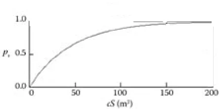
Assumption 3: “Tree vitality is good” is modeled
using the approach by PRETZSCH (2001). Vitality
depends on size of tree crown surface (cS) and tree
species. An example for beech is presented in Fig. 5. Vitality of beech is most sensitive to crown size.
Assumption 4: “Tree is alive” is modeled by
Bool-ean value (0 or 1). If the tree is dead, value is zero, otherwise value is one. Information about mortal-ity is modeled using a mortalmortal-ity model by ĎURSKÝ (1997).
The resultant score of existence for an individ-ual tree is calculated using the following equation (REYNOLDS 1999):
SCORE = MINP + (AVGP – MINP) × MINP (6)
MINP means minimal value of previous four
as-sumptions and AVGP means their average. The
re-sult is a value between 0 and 1. A tree has a greater probability of staying in the stand after thinning if
its SCORE is greater. Specific position has so-called
marginal score of existence. The marginal score can be fixed at a specific value, which we can then not exceed during selection. For example, if we specify a marginal score of 0.7 and we select thinning trees, we can not choose trees with a score than 0.7. If we select crop trees, we can not select trees with a score less than 0.7. The marginal value can be used to fix tree quality before execution of selection al-gorithms.
Model for type of selection
The modeling of selection depends on groups or sub-groups, because trees are selected within them.
In this case, a separator is established. The
separa-tor is a feature (characteristic) which classifies trees
into groups or sub-groups. The separator can be a qualitative value, a quantitative discrete value, or a quantitative continuous value. Bio-sociological status is an example of a qualitative value used in the thinning concept from below or above. Diameter class is an example of a quantitative discrete value in the thinning concept using target frequency curve (equilibrium curve). Target diameter or clearing ra-dius is an example of a quantitative continuous value used in the thinning concepts by target diameter and crop trees method.
With regard to groups and sub-groups, the
selection is performed by the following offered
ap-proaches. The sequential selection classifies trees
into groups and sub-groups. Then, the amount of harvesting trees is specified for all sub-groups together. Trees are selected step by step in a speci-fied sequence of sub-groups. As mentioned previ-ously, some sub-groups have higher priority. For example, in the thinning concept from below, trees have priority based on bio-sociological status as
follows: overshadow trees → intermediate trees →
co-dominant trees. We will indicate type of selection
by sub-groups separated by right arrow. Theparallel
[image:4.595.308.532.51.153.2]selection classifies trees into groups and sub-groups. Then, amount of harvesting trees is specified for all
[image:4.595.67.290.55.152.2]Fig. 5. Mathematical expression of assumption: Tree vitality is good (example for beech)
Fig. 3. Mathematical expression of assumption: Competition
[image:4.595.67.290.200.310.2]sub-groups together. Trees are selected simultane-ously from all subgroups. For example, crop trees are selected at the same time from dominant and co-dominant trees (co-dominant + co-co-dominant). We will indicate type of selection by sub-groups separated by
a plus symbol. Theserial selection classifies trees into
sub-groups. Then, the amount of harvesting trees is calculated individually for each sub-group. Selection is performed gradually with individual amounts for each sub-group. For example, the number of trees is reduced individually in diameter classes by a target
frequency curve (10, 14, ..., k). We will indicate type
of selection by sub-groups separated by comma. The limit selection distinguishes only one group, which is defined by a specific limit value. The selec-tion is performed only for this group. For example, trees having a diameter bigger than the limit value are harvested in target diameter thinning or trees within a specified radius are harvested around crop trees in the crop tree method. The first example is
over-limit selection and the second example is under-limit selection. We will indicate selection by upper arrow for over-limit selection and down arrow for
under-limit selection, for instance dmax↑ or Rmin↓. The
examples mentioned represent constant limit
selec-tion. There are also possibilities for variable limit
selection. For example, competitors are harvested which have a current distance from crop trees which is less than the marginal distance. Marginal distance is individual for each tree, depending on its A-value according to JOHANN (1982) and the dimensions of crop tree and competitor. We will indicate variable selection by a question mark in the upper index, in order to distinguish between constant and variable
selection, for instance: distij↓?. Theglobal selection
is a specific case in which we do not classify trees into any groups. Selection is performed from all trees in the stand. A typical example is degree of release for crop trees. Current A-values according to JOHANN (1982) are calculated for all trees in the stand. A-value depends on current distance between crop tree and competitor and their dimensions. Then, the necessary number of trees with the biggest A-values is removed. We will indicate selection with the symbol Ω.
The next important term for selection algorithms
is the selector. The selector is a feature
(character-istic), which help us to choose trees from groups or sub-groups. For example, score of existence is the most frequent selector. Trees are selected by their value in thinning from below, thinning from above, neutral thinning, crop tree method, target diameter method, and equilibrium curve method. Another example is the A-value by JOHANN (1982) at release
of crop trees by specified number of competitors. If we apply selection by selector in decreasing order,
then we call it positive selection. In the opposite
case, we call it negative selection. A specific case is
total selection, where we do not need any selector. We select all trees in the group. A typical example is harvesting all competitors around crop trees which are inside a clearing radius. In order to distinguish selections we use the following symbols:
:-) for positive selection, :-( for negative selection, and :-o for total selection (Tab. 3).
Model for amount of thinning
The algorithm for calculation of harvesting amount or specification of crop trees varies with thinning concept. We offer great scale of possibilities. If we combine type of selection with amount of thinning, we can model a lot of thinning concepts in a very flexible way.
Size of removal stand
Defining the amount of trees to be removed is one possibility to model thinning. We can use volume, basal area, or tree number for size of removal stand. The following variants are possible:
a) Thinning percentage (%VP) determines the relative volume to be harvested. Volume can be static or dynamic. Static volume percentage is a constant amount specified for the current period. Dynamic volume percentage is an amount that depends on age
(t), mean diameter (dg), mean height (hg), or dominant
height (h95%). We can select an appropriate function
for modeling dynamic volume. Offered functions for the SIBYLA model are in Table 1. Besides choosing a function, we must choose the type of independent
value (t, dg, hg, h95%) and estimate coefficients for the
function. Using of regression analysis outside of the SIBYLA model is convenient. We can modify the function by additivity and multiplier:
%V = Additivity + f(x) × Multiplier (7)
Default additivity is 0 and default multiplier is 1. We can modify these values, so the function is more flexible. Then, thinning percentage is transformed
into volume of removal trees (VP). Growing stock in
cubic meters before thinning (VZ) is utilized:
%Vp
Vp = Vz ––––– (8)
100
b) Development of remaining stand (YH = f(x))
is expressed by curve of growing stock (V/ha); basal
age (t), mean diameter (dg), mean height (hg), or
dominant height (h95%). We must choose an
ap-propriate function (Table 1), select dependent and independent values of the function, and specify the coefficients for the function. Amount of thinning
(YP) is calculated from size of stand before thinning
(YZ) using the function (f(x)), stand area (P), tree
spe-cies percentage (%R), and stand density (SD):
%R Yp = YZ – [Additivity + f (x) × Multiplier] . ––– × 100
× SD × P; valid for Yp > 0 (9)
c) Stand density of remaining stand (SD) is fixed by model
SD = Additivity + f (x) × Multiplier (10) The function, coefficient, and independent values are determined by the user. Then, volume of removal stand is calculated from growing stock before
thin-ning (VZ) and standard growing stock from yields
tables (VH(RT)) within the formula
%R
Vp = VZ – SD × VH(RT) ––– P; valid for Yp > 0 (11) 100
d) Volume of removal stand (VP) is the last vari-ant. This variant is the most simple and direct way to specify thinning amount. The variant is offered for purposes of forest updating if we know the actual amount of cuttings. This method can replace current updating methods, for example those by FABRIKA and ŠMELKO (2002).
Size of target group
A possibility is proposed for selection of crop trees. Number of crop trees is specified directly or indirectly by theoretical distance between crop
trees. Then, the resulting number of crop trees (NC)
is calculated by the following variants:
a) Number of crop trees (NC/ha). Simulation plot
area (P) and tree species percentage (%R) is used in
formula
%R
NC = (NC/ha) ––– P (12)
100
[image:6.595.59.533.70.437.2]b) Target distance between crop trees (aC). Number of crop trees is calculated by formula
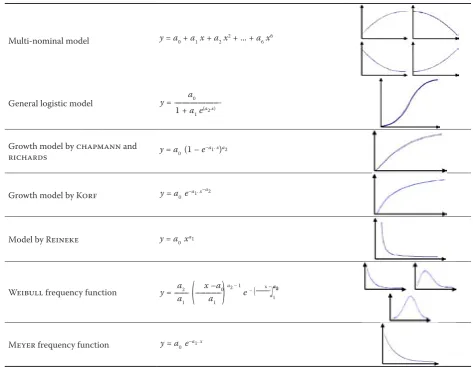
Table 1. Offered mathematical functions for description of thinning amount
Multi-nominal model
General logistic model
Growth model by CHAPMANN and RICHARDS
Growth model by KORF
Model by REINEKE
WEIBULL frequency function
MEYER frequency function
y = a0 + a1x + a2x2 + ... + a 6x6
a0
y = ——————
1 + a1 e(a2.x)
y = a0 (1 – e–a1. x)a2
y = a0 e–a1. x–a2
y = a0 xa1
a2 x –a0 x – a0
y = –––
(
–––––)
a2 – 1e– (–––––)a2 a1 a1 a1100
NC = ––– %RP (13)
aC2
Clearing radius
Clearing radius is offered for harvesting competi-tors in the crop tree method. The principle is very simple. We determine a fixed radius around crop
trees (Rmin). Competitors inside of the radius are
harvested without any reference to their dimensions, quality, or vitality.
Degree of release
This method represents another possibility for harvesting competitors in the crop tree method. The method is formulated in order to satisfy the requirements of the approach by SCHÄDELIN (1942) and ŠTEFANČÍK (1984) in their thinning concept. In this case, number of competitors is specified per crop tree. We harvest competitors with the biggest A-values according to JOHANN (1982):
H j di
A = ––– ––– (14)
aij Dj
where: Hj, Dj – height and diameter of crop tree,
di – diameter of competitor,
aij – distance between crop tree and competitor.
Marginal distance
Thinning amount is also modeled by JOHANN’S approach (1982) also. However, we determine A-value instead of competitors per crop trees.
Mar-ginal distance (distij) is calculated by
H j di
distij = ––– . ––– (15)
A Dj
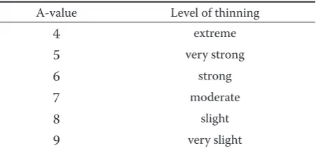
If real distance is less than marginal distance (aij < distij), then competitor is removed. JOHANN (1982) has defined different levels of thinning amounts (Table 2).
Target percentage
Target percentage is used in the target diam-eter method. We harvest a relative amount of trees
(%dmax) with diameter greater or equal to a specified
target dimension dmax. Number of thinning trees (NP)
is calculated by %dmax
Np = –––– n (di ≥ dmax) (16)
100
where: n(di ≥ dmax) – number of trees with diameter greater or equal to the target diameter.
Removal curve
A removal curve expresses the amount of har-vested trees in individual diameter classes. The SIBYLA model has two variants for specification of the removal curve:
a) Geometrical series by LIOCURT (1898). Target
harvesting dimension (dmax) and number of trees
with mentioned dimension (nd max) are inputs into
the model. In the first step, we calculate the mean quotient of the geometrical series by
i–1 i–1n
i
Σ
qiΣ
–– i=1 i=1 ni+1q = –––– = –––– (17)
i –1 i – 1
where: ni – numbers of trees in individual diameter classes.
We exclude extreme values of individual quotients
qi (less or qual to 1, bigger or equal to 2). Then we
calculate target frequency curve (equilibrium curve) by
mi = 10 [log ndmax] + (k – i) log q (18)
where: mi – target frequencies in diameter classes,
k – order for diameter class with target harvesting diameter dmax.
Number of trees harvested in individual diameter classes is calculated by
yi = ni – mi; valid for yi > 0 (19)
b) Regression model of frequency curve. A theo-retical frequency curve is input for the model. We can use for example WEIBULL function or MEYER function (Table 1):
m = Additivity + f(d1.3) × Multipier (20)
The resultant removal curve is calculated by
yi = ni – m(di) × h; valid for yi > 0 (21)
where: m(di) – number of trees in diameter class,
h – size of diameter class (standard is 4 cm).
Table 2. Level of thinning amount by A-value of JOHANN (1982)
A-value Level of thinning
4 extreme
5 very strong
6 strong
7 moderate
8 slight
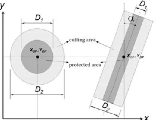
[image:7.595.306.532.648.754.2]Size of cutting element
This variant for calculation of thinning amount is developed mainly for stands in rotation period, but the model is also applicable to schematic or geomet-rical thinning. Amount of thinning is determined by cutting element (shape, size, and location). All trees inside the cutting element are harvested. We can use a circle cutting element or strip cutting element. The
circle is defined by coordinates (XOP, YOP) and
diam-eters (D1, D2). External diameter D1 means total size
of cutting element. Internal diameter D2 means area
protected against harvesting. This is very important if we want to extend circle cutting from a previous period and we want to save new trees established by natural regeneration in a previous cutting element. If we want to cut everything inside a circle, we specify
D1 equal to 0. We calculate the distances of all trees
from the middle of circle by
li =
√
(xi – XOP)2 + (yi – YOP)2 (22)
We remove all trees where distance:
D1 D2
–– ≤ li ≤ –– (23)
2 2
The strip is defined by coordinates for points on
the central axis (XOP , YOP) and by internal (D1) and
external (D2) width. Internal and external widths
have the same function as the circle diameters.
Rota-tion of the strip is defined by angleα from north. We
calculate the distances of all trees from the central axis by
– tg(90 – α) × xi + yi – [YOP – tg(90 – α) × XOP]
li =
|
–––––––––––––––––––––––––––|
(24)√ [– tg(90 – α)]2 + 1
We remove all trees according to the condition in formula 23.
Modeling thinning concepts
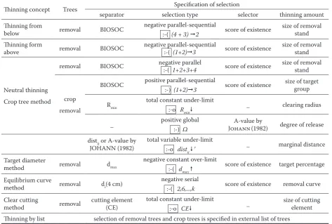
A lot of possibilities for thinning concepts are in-cluded in the SIBYLA model: thinning from below, thinning from above, neutral thinning, crop trees method, target diameter method, equilibrium curve method, clear cutting method, and method by list. The thinning algorithm is determined by separator, type of selection, selector, and method for calcula-tion of thinning amount. The modeling approach is summarized in Table 3.
Thinning from below
Negative parallel-sequential selection is used for this thinning method. At first, bio-sociological status and score of existence are calculated for individual trees. Bio-sociological status is the separator and
separates trees into sub-groups: overshadow with in-termediate trees (4 + 3) and dominant trees (2). Trees in sub-groups are arranged in ascending order by their score of existence. This means that score of ex-istence is the selector in this thinning method. Then, we calculate thinning amount using the approach
described in section Size of removal stand. Number
of removal trees is the result of the algorithm, but growing stock or basal area of removal stand are alter-native possibilities. It depends on user requirements. At a result, trees with the smallest score of existence are removed (negative selection) from sub-groups. The process of removing is parallel in sub-groups 4 + 3 and if removal amount is not sufficient, process continues sequentially in sub-group 2. Removal of thinning trees is repeated until the thinning amount is reached. We can use also marginal score of exist-ence and fix the quality of remaining trees. In this case, we can not exceed a specified score of existence during the process of tree selection.
Thinning from above
This thinning method is modeled by an approach that is similar to the previous one. Negative paral-lel-sequential selection is utilized, BIOSOC value is used as separator, and score of existence is used as a selector. Amount of thinning is calculated by size of removal stand. However, different sub-groups
and their order is formulated: (1 + 2) → 3. We can
use also marginal score of existence in order to fix tree quality.
Neutral thinning
This method is modeled by negative parallel se-lection. The BIOSOC is the separator. The score of existence is the selector and can be fixed by marginal value. Thinning amount is calculated by the same procedure as in the previous methods. However, score of existence is ordered in a frame of all bio-sociological layers together (1 + 2 + 3 + 4). Then, selection is parallel in all layers at the same time. The layers have the same priority. Therefore, the thinning method is neutral.
Crop tree method
This method is modeled in two phases. We select crop trees in the first phase and competitors in the
second phase. Selection of crop trees is done with
positive parallel-sequential selection. The bio-so-ciological status is the separator and the score of existence is the selector. Size of selection is defined
by the procedure described in the section Size of
descending order by score of existence (positive se-lection). This means that the best trees are selected. Sub-groups and their order are the same as in thin-ning from above. We can also use marginal score of
existence and fix crop tree quality. Selection of
com-petitors is modeled by three different alternatives. The first alternative is total constant under-limit
selection. Clearing radius (Rmin) around crop trees is
[image:9.595.62.536.75.394.2]defined as separator. The radius separates trees into a group inside the circle and a group outside the circle.
Table 3. Modeling of thinning concepts
Thinning concept Trees Specification of selection
separator selection type selector thinning amount Thinning from
below removal BIOSOC negative parallel-sequential :-( (4 + 3) 2 score of existence size of removal stand Thinning form
above removal BIOSOC negative parallel-sequential :-( (1+2)3 score of existence size of removal stand
Neutral thinning Crop tree method
removal BIOSOC negative parallel :-( 1+2+3+4 score of existence size of removal stand
crop removal
BIOSOC positive parallel-sequential
:-) (1+2)3 score of existence
size of target group
Rmin total constant under-limit
:-o Rmin _ clearing radius
_ positive global
:-) Ω JOHANNA-value by (1982) degree of release distij or A-value by
JOHANN (1982) total variable under-limit :-o distij ? _ marginal distance Target diameter
method removal dmax
negative constant over-limit
:-( dmax score of existence target percentage Equilibrium curve
method removal di(4 cm)
negative serial
:-( 2,6,...,k score of existence removal curve
Clear cutting
method removal cutting element (CE) total constant under-limit :-o CE _
size of cutting element Thinning by list selection of removal trees and crop trees is specified in external list of trees :-) for positive selection, :-( for negative selection, and :-o for total selection
[image:9.595.76.518.535.720.2]All trees inside the circle are competitors and are removed. The second alternative is positive global selection. An A-value according to JOHANN (1982) is calculated for each tree, considering all crop trees. Equation 14 is applied. The user specifies the number of competitors per crop tree and the algorithm se-lects this number of trees. Trees with the biggest A-value are selected. The third alternative is total variable under-limit selection. We determine thin-ning power by A-value (Table 2). Marginal distance
(dij) is calculated for each tree, considering all crop
trees. Equation 15 is applied. The marginal distance is the limit. All trees with real distance to crop trees less than marginal distance are removed.
Target diameter method
This method is modeled by negative constant over-limit selection. Target diameter and target percentage are user inputs into the model. First, selector values (score of existence) for each tree are calculated. Then, we calculate number of removal trees using equation 16. Trees are separated into two groups: trees with diameter less than target diameter and trees with diameter bigger or equal to target diameter. Trees in the second group are organized in ascending order by score of existence. At last, we remove the necessary number of trees with smallest score of existence. Marginal score of existence is rejected from the algorithm.
Equilibrium curve method
This method is modeled by negative serial selec-tion. At first, we calculate score of existence for each tree. The score of existence is the selector. Then, we classify trees into diameter classes with size 4 cm. Di-ameter class is the separator. Afterwards, we
calcu-late number of removal trees in diameter classes. We can use geometrical series (equation 18) or external function (equation 20). Trees in individual diameter classes are ranked by score of existence. We remove the necessary number of trees with the smallest score of existence in each diameter class. Marginal score of existence is rejected from the algorithm.
Clear cutting method
This method is modeled by total under-limit selec-tion, which means that all trees with co-ordinates inside the cutting element are harvested. The user specifies the cutting element (circle or strip) using Fig. 7. Distances from the center of the cutting ele-ment are calculated for each tree. Trees, which fulfill condition 23, are removed. Minimal tree height is an additional property. We can utilize this height as a limit for cutting. If tree height is less than the mentioned height, the tree is not harvested. The limit is very important for protecting natural rege-neration.
Thinning by list
[image:10.595.78.349.551.753.2]The last thinning method is specific, because method is fully controlled by user. Trees are not selected by algorithm. The user specifies selection in an external list of removal and crop trees. This method is very important for updating research plots. We have repeated measurements with tree coordinates and stem and crown parameters on per-manent research plots. We usually have information about removed or dead trees from previous years and sometimes have information about crop trees. We can prepare a list and execute growth prognosis. Afterwards we can compare the real situation on the plots with the situation from the prognosis. In this
manner we can evaluate and calibrate growth models in a very flexible way. Another example for usage is an e-learning process. Students can use virtual real-ity for visualization of forest stand (FABRIKA 2003b) and can do interactive thinning in virtual stands. All marked trees (removal and crop trees) are saved into the list of trees. The list is used as input for the growth model SIBYLA. In this case, growth models and this thinning method can serve as a tool for training of thinning skill in forestry education.
RESULTS AND DISCUSSION
The real stand 285A from the Forest District of the Technical University in Zvolen has been chosen for thinning model presentation. The stand belongs to forest type 410 (fresh beech stands) and stand type 22 (beech stands with spruce and fir). We have uti-lized stand data from forest inventory (1993) in order to reconstruct initial stand structure. The stand is 45 years old. Stand area is 8.22 ha and stand density is 0.9. The stand is situated at west aspect with slope
50%. Total growing stock is 2,474 m3, which is 301 m3
[image:11.595.68.533.57.403.2]per ha. Spruce, fir, oak, and hornbeam exist in the
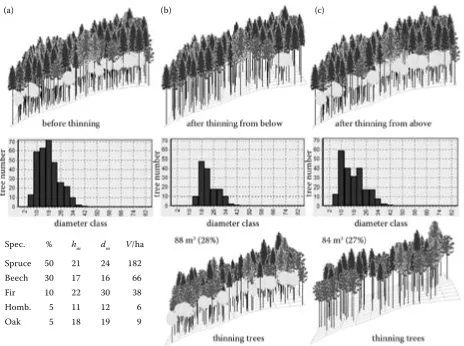
Fig. 8. Example of thinning from below and thinning from above: (a) before thinning, (b) after thinning from below, (c) after thinning from above
stand. Tree species composition (percentage) and quantitative characteristics (mean height, mean di-ameter, volume per ha) are in table in Fig. 8. We have generated individual tree information (diameters, heights, quality, crown parameters, and coordi-nates) from forest inventory data. Methodology of PRETZSCH (2001) has been applied. We generated a square plot with size 0.25 ha. After generation of the
structure, the plot includes 315 m3 per ha with mean
diameter 21 cm and mean height 19 m. Total
grow-ing stock is distributed as follows: spruce 192 m3,
beech 69 m3, fir 41 m3, oak 7 m3, and hornbeam 6 m3.
This means that the simulation plot is almost equal to its sample from forest inventory. Moreover, the simulation plot has been located on a digital terrain model using the methodology of PAPAJ (2004) and vertical tree coordinates have been derived using the methodology of FABRIKA (2003b).
We have chosen thinning from below and thinning from above as a first example of thinning concepts. Thinning amount is the same in both cases. We used a standard thinning percentage from Slovakian for-est management according to HALAJ et al. (1986). Percentage depends on species and stand age. The
(a) (b) (c)
Spec. % hm dm V/ha Spruce 50 21 24 182 Beech 30 17 16 66
Fir 10 22 30 38
amount is derived for thinning at intervals of one
time per ten years. Generally, we removed 88 m3
(28%) in thinning from below and 84 m3 (27%) in
thinning from above. The thinning concept results are shown in Fig. 8. The stands and their diameter distributions are shown in the picture. In addition, harvested trees are drawn separately for both thin-ning concepts. Frequency functions for thinthin-ning concept are left asymmetrical, low diameter classes are reduced in thinning from below, and upper diam-eter classes are reduced in thinning from above.
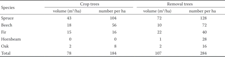
As a second example, we have applied the crop tree method. We specified 200 crop trees per ha with mean distance of approx. 7 m. We have chosen the degree of release method, with 2 competitors per crop tree. The results of the thinning method are
presented in Fig. 9 and Table 4. We removed 107 m3
per ha, or 34% of the initial growing stock. The speci-fied number of crop trees is not satisspeci-fied, because hornbeam does not meet the criteria for crop trees. In total 4 trees in the plot have not been accepted and it is 16 trees per ha. This is the same number, which absents to 200 trees per ha.
The proposed thinning model represents a com-plex solution of thinning tools for the SIBYLA growth simulator. The model includes each of the important thinning concepts in Slovakia and allows very flexible combinations of thinning type, thin-ning volume, and thinthin-ning interval. The model is developed especially for SIBYLA software, because the SILVA software does not include all specific
requirements for Slovakian conditions. The SILVA model does not consider tree quality in the thinning model. Tree quality is very important for thinning concepts in Slovakia and it is estimated in regular forest inventory measurements.
The advantages of SIBYLA thinning model com-pared to the SILVA model are the following:
– Period of thinning is optional, minimum one year. The SILVA model is fixed to a five-year period. – Thinning concepts can be variable for each period
and each tree species. Thinning concepts in SILVA are fixed to stand development stage (defined by dominant height) and must be the same for all tree species.
– Thinning amount is more flexible. We can use also volume and stand density, not only tree number and basal area like in SILVA. Development of the values also depends on mean diameter, mean height, and dominant height, not only on age as in SILVA.
– We can use a lot of functions: multi-nominal function, logistic function, functions by CHAP-MANN and RICHARDS, KORF, REINEKE, WEIBULL, and MEYER. In the SILVA model, we can use only multi-nominal function.
– We consider tree quality and tree vitality in the thinning model by score of existence. The SILVA model does not support these parameters in thin-ning concepts.
[image:12.595.68.530.60.317.2]– Some thinning concepts are based on bio-socio-logical tree status and therefore are more similar
Fig. 9. Example of thinning by crop tree method: (a) before thinning, (b) after thinning, (c) only crop trees (c)
to real thinning concepts in forestry practice. The SILVA model does not classify trees into a bio-sociological scale.
– Crop trees are defined in a more flexible way. We can use also target distance between crop trees as input. Also, we can specify a new selection of crop trees or we can use crop trees marked in previ-ous thinning concepts. This means that we can emulate thinning concepts by SCHÄDELIN (1942) and ŠTEFANČÍK (1984). They use two categories of crop trees (expectant and target). The first category is fixed in the stand at a young age and moves to the second category only in older age. – We offer new thinning concepts: neutral thinning,
method of equilibrium curve for selection forest, clear cutting method for next artificial or natural regeneration, and thinning by list for forest updat-ing on permanent research plots.
– The tool for interactive thinning by virtual reality (FABRIKA 2003b) is built directly into the SIBYLA model. In this case, we can use the SIBYLA model directly in an e-learning process without restric-tions. The SILVA model offers interactive thinning only by external tools, for example with TreeView from SEIFERT (1998). Reverse connection to growth simulator is applied only by external data pre-processing with user assistance.
– Dead trees are not removed in the stand automati-cally in thinning measures. User can decide if he wants cut them during thinning or leave them in the stand. We cut only these trees which are necessary. This approach protects forest biodiver-sity by saving dead wood in the stand. Sanitation thinning is liable in the stand. In this case, we must select a concept without thinning and with harvesting of dead trees.
The SIBYLA model has some disadvantages com-paring to the SILVA model:
– Internal definition for degree of thinning power is not implemented in the SIBYLA model. For example, qualitative levels of thinning are defined in the SILVA model (slight, medium or strong) or
thinning by optimal basal area (ASSMANN 1961) is offered. The user defines thinning amount in the SIBYLA model with external functions. The user must determine the type of function, independent and dependent values, and coefficients. This is flexible, but not so user friendly.
– Interval for thinning is fixed to age. The SILVA model offers size of dominant height increment as one possibility for thinning execution, for example after each 3 m of height increment.
– In conclusion, we can say that the proposed thin-ning models represent a considerable contribu-tion to thinning modeling and forest prognosis in Slovakia. Because, no thinning model existed in Slovakia before, we can regard the result as very significant.
References
ASSMANN E., 1961. Waldertragskunde. München, Bonn, Wien, kdo vydal: 490.
DAUME S., ROBERTSON D., 2000. A heuristic approach to model thinnings. Silva Fennica, 34: 237–249.
ĎURSKÝ J., 1997. Modellierung der Absterbeprozesse in Rein- und Mischbeständen aus Fichte und Buche. Allgemeine Forst- und Jagdzeitung, 168: 131–134.
FABRIKA M., 2003a. Rastový simulátor SIBYLA a možnosti jeho uplatnenia pri obhospodarovaní lesa. Lesnícky časopis – Forestry Journal, 49: 135–151.
FABRIKA M., 2003b. Virtual forest stand as a component of sophisticated forestry educational system. Journal of Forest Science, 49: 419–428.
FABRIKA M., ŠMELKO Š., 2002. Aktualizácia stavu lesa a jej spresnenie kontrolným výberovým meraním. Acta Facul-tatis Forestalis Zvolenensis, XLIV: 143–156.
HALAJ J., 1985. Kritické zakmenenie porastov podľa nových rastových tabuliek. Lesnícky časopis, 31: 267–276. HALAJ J., PETRÁŠ R., SEQUENS J., 1986. Percentá prebierok
pre hlavné dreviny. Lesnícke štúdie VÚLH Zvolen. Bratis-lava, Príroda: 98.
[image:13.595.65.531.73.191.2]HALAJ J. et al., 1987. Rastové tabuľky hlavných drevín ČSSR. Bratislava, Príroda: 361. (citovat v textu)
Table 4. Results of crop tree thinning for stand 385A
Species Crop trees Removal trees
volume (m3/ha) number per ha volume (m3/ha) number per ha
Spruce 43 104 72 128
Beech 18 56 10 72
Fir 15 16 22 40
Hornbeam 0 0 1 28
Oak 2 8 2 16
JOHANN K., 1982. Der “A-Wert” – ein objektiver Parameter zur Bestimmung der Freistellungsstärke von Zentralbäu-men. Bericht von der Jahrestagung der Sektion Ertrags-kunde im DVFFA in Weibersbrunn: 146–158.
KAHN M., 1995. Die Fuzzy Logik basierte Modellierung von Durchforstungseingriffen. Allgemeine Forst- und Jagdzei-tung, 166: 169–176.
KONŠEL J., 1931. Stručný nástin tvorby a pěstění lesů v bio-logickém ponětí. Písek, kdo vydal: 552.
KORPEĽ Š., PEŇÁZ J., SANIGA M., TESAŘ V., 1991. Pesto-vanie lesa. Bratislava, Príroda: 465.
LEDERMANN TH., 2002. Using Logistic Regression to Model Tree Selection Preferences for Harvesting in Forest in Con-version. In: VON GADOW K., NAGEL J., SABOROWSKI J. (eds.), Managing Forest Ecosystems: Continuos Cover For-estry – Assessment, Analysis, Scenarios, Vol. 4. Dordrecht, Boston, London, Kluwer Academic Publisher: 203–216. LIOCURT F. DE., 1898. De ľaménagement des sapiners.
Bul-letin of the Soc.vypsat Forest. Franche-Comté et Belfort,
4: 396–409.
MEYER H.A., 1952. Structure, growth and drain in balanced uneven-aged forests. Journal of Forestry, 50: 85–92. PAPAJ V., 2004. Využitie digitálneho modelu terénu pri vizuali-
zácii lesných porastov a rastových simuláciách. [Diplomová práca.] Zvolen, TU: 86.
PETRÁŠ R., NOCIAR V., 1990. Nové sortimentačné ta-buľky hlavných listnatých drevín. Lesnícky časopis, 36: 535–552.
PETRÁŠ R., NOCIAR V., 1991. Nové sortimentačné ta-buľky hlavných ihličnatých drevín. Lesnícky časopis, 37: 377–392.
PRETZSCH H., 2001. Modellierung des Waldwachstums. Berlin, Parey Buchverlag: 341.
REMIŠ J. et al., 1988. Modely a technologické postupy pre fá-zové výrobky pestovnej činnosti. Bratislava, Príroda: 110. REYNOLDS K.M., 1999. NetWeaver for EMDS user guide
(version 1.0): a knowledge base development system. Gen. Technical Report? PNW-GTR-XX. Portland, OR. U.S. De-partment of Agriculture, Forest Service, Pacific Northwest Research Station: XX.
SEIFERT S., 1998. Dreidimensionale Visualisierung des Wald-wachstums. [Diplomarbeit im Fachbereich Informatik der Fachhochschule München in Zusammenarbeit mit dem Lehrstuhl für Waldwachstumskunde der Ludwig-Maximil-lians-Universität München.] München: 133.
SCHÄDELIN W., 1942. Die Ausledurchforstung als Erzie-hungsbetrieb höchster Wertleistung. Bern, Leipzig, kdo vydal, stránky.
ŠTEFANČÍK L., 1974. Prebierky bukových žrďovín. Lesnícke štúdie, VÚLH Zvolen, 20: 141.
ŠTEFANČÍK L., 1977. Prečistky a prebierky v zmiešaných smrekovo-jedľovo-bukových porastoch. Lesnícke štúdie, VÚLH Zvolen, 25: 89.
ŠTEFANČÍK L., 1984. Úrovňová voľná prebierka – metóda biologickej intenzifikácie a racionalizácie selekčnej vý-chovy bukových porastov. Vedecké práce VÚLH Zvolen: 69–112.
Received for publication June 1, 2005 Accepted after corrections July 13, 2005
Algoritmus a softwarové riešenie prebierkového modelu rastového simulátora
SIBYLA
M. FABRIKA, J. ĎURSKÝ
Lesnícka fakulta, Katedra hospodárskej úpravy lesov a geodézie, Technická univerzita vo Zvolene, Zvolen, Slovenská republika
ABSTRAKT: Práca sa zaoberá návrhom prebierkového modelu pre rastový simulátor SIBYLA. Model je založený na ana-lyticko-kauzálnom prístupe, pričom niektoré čiastočné hypotézy a modely sú preverené na podklade experimentálnych údajov pochádzajúcich z prebierkových pokusov. Samotný model sa skladá z nasledujúcich modelových zložiek: modelu biosociologického postavenia stromu, modelu existenčného skóre, modelovania druhu výberu, modelovania sily zásahu a napokon agregovaného modelu druhu prebierky. Vhodnou kombináciou druhu výberu a definovania sily zásahu je možné uskutočniť nasledujúce prebierky: podúrovňová prebierka, úrovňová prebierka, neutrálna prebierka, metóda budúcich rubných stromov, metóda cieľovej hrúbky, metóda cieľovej frekvenčnej krivky, metóda obnovného prvku a prebierka podľa zoznamu (resp. interaktívna prebierka). V závere je uvedené softwarové riešenie na príklade rôznych prebierkových režimov vo vybranom lesnom poraste a sú rozobraté výhody a nevýhody modelov oproti prebierkovému modelu rastového simulátora SILVA.
V súčasnosti sa v lesníctve a v ekológii neustále výraznejšie presadzujú pri modelovaní rastu lesných ekosystémov stromové rastové modely. V prípade, ak chceme tieto modely zaviesť aj do oblasti bežnej lesníckej prevádzky, musia modely disponovať aj ná-strojmi pre modelovanie prebierkových zásahov. Au-tomatický výber prebierkových stromov na základe stanovenia druhu, sily a intervalu prebierky potom umožní voliť rôzne stratégie obhospodarovania lesa a podporí výber optimálneho variantu.
V rokoch 2001–2004 prebiehal na Slovensku vývoj stromového rastového simulátora SIBYLA (FABRIKA 2003a), ktorý bol podporený Európskou komisiou v rámci 5. rámcového programu Európskej únie. Neskôr bol do modelu zabudovaný nový prebierkový nástroj (thinning engine). Jeho vývoj bol financovaný nadáciou ALEXANDRA VON HUMBOLDTA v rokoch 2004 a 2005 počas pôsobenia jedného z autorov na Univerzite Georga-Augusta v Göttingene. Prebier-kový model je založený na analyticko-kauzálnom prístupe. Model sa skladá z nasledujúcich kom-ponentov: modelu bio-sociologického postavenia stromu (model BIOSOC), modelu existenčného skóre stromu, modelu druhu výberu, modelu pre-bierkovej sily a napokon modelu druhu prebierky. Bio-sociologické postavenie stromu je modelované pomocou klasifikačného pravidla (vzťah 3). Klasifi-kačné pravidlo je založené na výpočte hornej výšky a na stanovení osvetlenej a zatienenej časti koruny stromu s hornou výškou (obr. 1). Existenčné skóre stromu (od 0 po 1) indikuje jeho uprednostnenie do ťažby (ak je blízke 0), alebo podporu v rámci
skupiny budúcich rubných stromov (ak je blízke 1). Do modelu existenčného skóre (vzťah 6) vstupuje konkurenčný tlak stromu (obr. 3), kvalita stromu (obr. 4), vitalita stromu (obr. 5) a mortalita stromu. Výber stromov je prevádzaný prostredníctvom na-sledujúcich druhov výberu: sekvenčný, paralelný, sériový, limitný a globálny. Výber sa uskutočňuje vo vnútri skupín a podskupín stromov, ktoré sú defino-vané pomocou klasifikačného znaku (separátora), alebo sa výber prevádza v rámci celého porastu (simulačnej plochy). Výber môže byť zabezpečený negatívnym, pozitívnym alebo totálnym prístupom pomocou zvoleného výberového znaku (selektora). Sila prebierky je modelovaná pomocou nasledujú-cich variantov: veľkosti podružného porastu, veľ-kosti cieľovej skupiny, polomeru uvolnenia, stupňa pomoci, hraničnej vzdialenosti, cieľového percenta, krivky odberu alebo veľkosti obnovného prvku. Vhodnou kombináciou druhu výberu a prebierkovej sily (tab. 3) dosiahneme realizáciu nasledujúcich prebierkových konceptov: podúrovňová prebierka, úrovňová prebierka, neutrálna prebierka, metóda budúcich rubných stromov, metóda cieľovej hrúb-ky, metóda cieľovej frekvenčnej krivhrúb-ky, metóda obnovného prvku a prebierka podľa zoznamu, resp. interaktívna prebierka.
Uvedený prebierkový model predstavuje kom-plexné riešenie prebierkového nástroja pre rastový simulátor SIBYLA. Zahŕňa všetky dôležité prebier-kové postupy používané na Slovensku a zároveň umožňuje veľmi flexibilnú kombináciu druhu, sily a intervalu prebierkových zásahov.
Corresponding author:
Ing. MAREK FABRIKA, Ph.D., Technická univerzita vo Zvolene, Lesnícka fakulta, Katedra hospodárskej úpravy lesov a geodézie, T. G. Masaryka 24, 960 53 Zvolen, Slovenská republika