The K Value Distribution of Liquid Phase Sintered Microstructures

Full text

(1)Materials Transactions, Vol. 43, No. 8 (2002) pp. 2115 to 2119 c 2002 The Japan Institute of Metals. The K Value Distribution of Liquid Phase Sintered Microstructures Po-Liang Liu ∗ and Shun-Tian Lin Mechanical Engineering Department, National Taiwan University of Science and Technology, Taipei City, Taiwan, 106, R. O. China A complex geometry of a powder compact in the three-dimensional multiple particle arrangement was generated by a Monte Carlo method, and the K value (a constant links the two-dimensional connectivity to the three-dimensional coordination number) distributions of liquid phase sintered systems, parameters linked the two-dimensional connectivity to the three-dimensional coordination number, were solved by the numerical computation. With this probability model, irregular packing of particles in three-dimensional space could be formulated with the variations of the particle size distribution. Unlike previous analytical models in which the grain boundary energy was set to a constant value, a relationship between the grain boundary energy and the misorientation angle between neighboring grains could be incorporated into this model in a probability manner. Simulation results indicate that the mean K value in the initial stage of liquid phase sintering increases with an increasing volume fraction of liquid phase, an increasing ratio of the mean base particle size to the mean additive particle size, and a decreasing standard deviation of the particle size distribution. The findings of the simulation are favorably compared with previous experimental observations on W–Ni–Fe alloys. (Received February 5, 2002; Accepted June 11, 2002) Keywords: K value; Monte Carlo model, coordination number, connectivity, grain boundary energy, dihedral angle. 1. Introduction The coordination number is determined by the number of contacts per solid grain in a three-dimensional (3-D) space. Sintered microstructures include a distribution of coordination numbers. The coordination number distribution is an important descriptor of the short-range spatial arrangement of grains, and it determines the grain connectivity and structural rigidity in a 3-D microstructure.1) The coordination number has been frequently studied to elucidate a true 3-D microstructure during liquid phase sintering, and thus reveals the microstructural effects on the distortion and segregation of solids and liquids.2–5) For example, Y. Liu et al. reported that, in a liquid phase sintered system in which the density of the solid differs significantly from that of the liquid, the mean coordination number is influenced by gravity, and varies systematically with the distance from the top of the specimen.5) Furthermore, recent works by A. Tewari et al. used a montage serial sectioning to reconstruct a 3-D microstructure of a 83 mass%W–Ni–Fe alloy.1) The author has provided a bivariate distribution of 3-D coordination numbers that expresses the fraction of grains having a given coordination number and having a size in a certain range. Microstructural analysis of 3-D coordination numbers has grown over recent years. There are two main methods applied to determine the 3-D coordination number. First, previous works were typically used the Monte Carlo method based on the two-sphere model to quantify the correlation between the 3-D coordination number and the two-dimensional (2-D) connectivity.2) They found that the 3-D coordination number ∞. N̂ can be related to the 2-D connectivity C and the dihedral angle Ψ by the following expression: ∞. C = K N̂ sin(Ψ/2),. (1). where K is a constant, which depends on the grain size dis∗ Present. address: Department of Mechanical Engineering, Tung Nan Institute of Technology, Taipei, 22202, Taiwan, R. O. China.. tribution, dihedral angle, and volume fraction of solid phase. They found K = 0.81 which was performed for monosized grains, six different packing coordinations of 1, 2, 4, 6, 8, and 12, and dihedral angles of 15 deg up to 75 deg.2) Due to the difficulty in the observation of the true 3-D coordination number, the 2-D connectivity is proposed. Therefore, K values are important factors which link the 2-D connectivity to the 3-D coordination number. However, little research has been devoted to the K value distribution. Second, a few works recently discussed on the montage based serial sectioning method to reconstruct a 3-D microstructure of a tungsten heavy alloy.1) In this investigation, distributions of 3-D coordination numbers are observed in the opaque microstructures. The disadvantage of this investigation is the difficulty in dealing with a great number of 2-D metallographic sections for a given alloy. There are a number of experimental results associated with the 2-D connectivity and the dihedral angle, mainly the easy observation in measuring the grain boundaries in a typical 2-D metallographic cross section. Therefore, a possible K value distribution plays a significant role predicted the true 3-D coordination number. In summary, this study aims to provide a possible K value distribution according to the rules of logic based on the theoretical and experimental investigations. Recently, the present authors developed a 3-D multiparticle model which can simulate a microstructure of liquid phase sintering where an anisotropy in grain boundary energy, different particle sizes and solid volume fractions are employed.6) In this study, the contacts per particle in a 2-D cross section is added to offer a possible K value distribution. In order to confirm the present model, the distribution is applied to tungsten grains in a W–Ni–Fe alloy during the initial stage of liquid phase sintering. The 3-D coordination number of tungsten grains in liquid phase sintered heavy alloy specimens is determined. According to the present results for the K value distribution, and the 2-D connectivity and the dihedral angle in a typical 2-D metallographic cross section, solving the eq. (1) yields the 3-D coordination number of tung-.

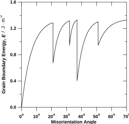
(2) P.-L. Liu and S.-T. Lin. 2. Model Geometry The simulation of a 3-D multi-particle arrangement incorporated the interface energy spectrum employs an identical procedure to that previously developed by the present authors.6) It assumed that base powders and additive powders in the powder compact are mixed and packed together. Mixed powders are heated to a temperature at which liquid forms in sintering. These powders are assumed to be spherical particles. In this model, all particles are assumed to bond together during heating, prior to liquid formation. The additive particles are assumed to melt into the liquid phase at the sintering temperature. A realistic model is generated by employing powders of the liquid (additive powders) and solid phases (base powders) whose particle size distributions exhibit truncated normal distributions. In the truncated normal distribution, only the particle sizes situating in the interval between R−3σ and R+3σ are generated in the calculation, where R is the mean particle radius and σ is the standard deviation of the distribution. The distribution function is denoted by Ň (R, σ ). Four different particle size distribution functions representing different mean particle sizes and different standard deviations were assumed (Fig. 1), and different combinations of liquid phase and solid phase particles were employed for simulation. In addition, monosized particles, Ň (R, 0), were also employed for simulation in the present investigation. The relative volumetric ratios of solid phase to liquid phase, designated 25, 50, 75, and 90 vol% solid phase particles with the remainder of the liquid phase particles, were treated as input variables that determined their relative probabilities in probabilistic generation of particles. Each particle was randomly generated according to the size distribution functions of solid and liquid phases, and the relative volume fraction of each phase. In liquid phase sintered systems, solid grains can either exist as isolated grains or bond with the adjacent grains, which accordingly yields a distribution of dihedral angle.. Anisotropy in grain boundary energy causes such a phenomenon. In fact, the grain boundary energy between two adjacent grains is determined by the misorientation angle of these two grains. According to the previous papers, the relation between the measured grain boundary energy of tungsten and the misorientation angle can be expressed in Fig. 2.7, 8) Bonding of adjacent grains occurs prior to the formation of liquid phase. When the liquid phase is formed, it causes to dissolve the grain boundary under the following thermodynamic criterion. 2χsl ≤ χGB ,. where χsl and χGB respectively denote the energy of a solidliquid interface and the grain boundary energy.9–13) If the grain boundary energy is smaller than twice the energy of the solid-liquid interface during liquid phase sintering, the liquid dose not penetrate and dissolve the grain boundary. Under such a condition, there will exist an equilibrium dihedral angle Ψ among the solid grains and the liquid phase (Fig. 3), which can be expressed by: χGB = 2χsl cos(Ψ/2).. 1.6. 1.2. 0.8. 0.4. 0.0 o. 10. o. 20. 0.5. N (8, 1). (3). Herein, the energy of a solid(W)-liquid(Ni–Fe) interface, χsl , is taken as 0.55 J/m2 .14). 0. N (4, 1). (2). -2. sten grains. The result of this study should simplify the task of finding the 3-D coordination number of tungsten grains.. Grain Boundary Energy, E / J . m. 2116. o. o. o. 30 40 50 Misorientation Angle. o. 60. o. 70. o. Fig. 2 Tungsten grain boundary energy spectrum.7, 8). N (16, 1). Probability Density. 0.4. Liquid phase 0.3. Grain boundary. N (8, 2). 0.2. 0.1. Solid particle. Solid particle. 0.0. 0. 4. 8. 12. 16. 20. Particle Size, r/ m Fig. 1 Four distributions describing sharpness of particles used in this work.. Fig. 3 The dihedral angle between two intersecting solid particles with a partially penetrating liquid phase..

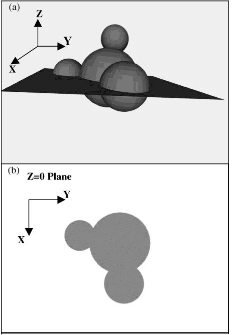
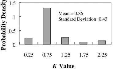
(3) The K Value Distribution of Liquid Phase Sintered Microstructures 0.8. 2117. (a). Mean = 1.19 Standard Deviation = 0.44. 0.6 0.4 0.2 0 1.5. (b). Mean = 0.97 Standard Deviation = 0.44. 1. Probability Density. 0.5 0. 1.5. (c). Mean = 0.82 Standard Deviation = 0.41. 1 0.5 0. 1.5. (d). Mean = 0.71 Standard Deviation = 0.33. 1 0.5 0 Fig. 4 Sketch of contacts per particle in (a) a three-dimensional space and (b) a two-dimensional cross section.. The packing coordination number of each central particle is determined in the model shown in Fig. 4. To determine the mean contacts per grain in a 2-D cross section, it is assumed that the x–y plane at z = 0 is a typical 2-D metallographic cross section. Neighboring contacts of each base particle in this 2-D cross section are determined. Furthermore, the probability model determines the effect of system thermodynamics (χGB /χsl ) on the dihedral angle during liquid phase sintering. The model’s basic operation generates a random misorientation, which is applied to the specified grain boundary between two-bonded particles, to determine the grain boundary energy. Grain boundaries with the lowest boundary energy are more likely to be formed by the rotation of particles, which is not considered in this analysis. If the grain boundary energy is smaller than twice the energy of the solid-liquid interface during liquid phase sintering, solving the eq. (3) will calculate the dihedral angle. With the above definition, the K value can be calculated by using the eq. (1). 3. Numerical Simulation The Monte Carlo method provides approximate solutions to a possible K value distribution by performing statistical sampling experiments on a computer. The program was run on a workstation of the SunOS Release 4.1.3 of the UNIX system using SIMCRIPT as the computer programming language. The Monte Carlo method is best suited for representing complex simulation models. Statistical comparisons of. 0.25. 0.75. 1.25. 1.75. 2.25. K Value Fig. 5 The effect of volume fractions of solid on K value distributions for Ň (8, 2) particle size distributions: solid volume fractions (a) 25%, (b) 50%, (c) 75%, and (d) 90%.. 1000 simulated grains were made between the present results of the two effects of the volume fraction of solid phase and the particle size distribution during the initial stage of liquid phase sintering. Subsequently, the results by numerical computation are briefly discussed. 4. Results and Discussion The simulations were performed for four different particle size distributions and monosized particles, and solid volume fractions of 25, 50, 75, and 90 vol%. Figure 5 reveals histograms for K value distributions of specimens with different solid volume fractions for Ň (8, 2) base and additive particle size distributions. According to our results, the mean of the K value distribution increases with an increase in the volume fraction of liquid phase, mainly due to the decreasing of the probability of particle contacts. Figure 6 displays histograms for K value distributions of specimens of solid volume fractions of 90 vol% for various ratios of the mean base particle size to the mean additive particle size. The majority of small base particles with some large additive particles have an advantage contributing to the probability of particle contacts. The mean of K value distributions for a given volume fraction of solid decreases with an increase in the probability of parti-.

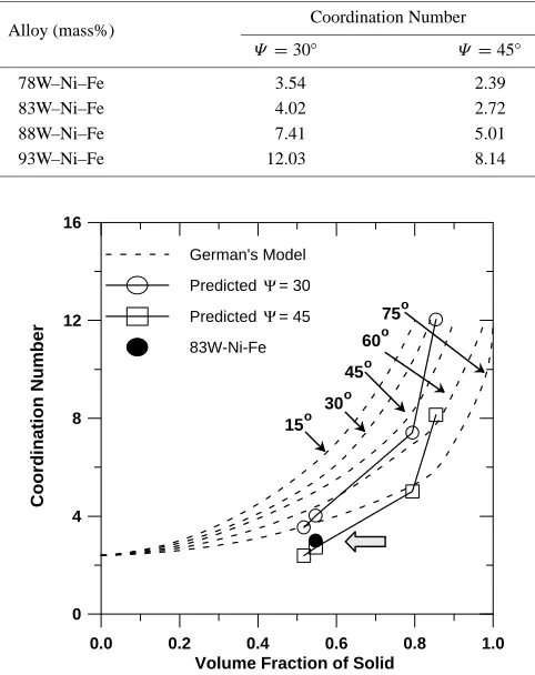
(4) 2118. P.-L. Liu and S.-T. Lin 1. 1.6. (a). Base Particles:Additive Particles N (4,1): N (8,1) N (8,2): N (8,2) N (8,1): N (8,1) N (8,0): N (8,0) N (16,1): N (8,1). Mean = 0.69 Standard Deviation= 0.40. 0.8 0.6. 1.4. 0.4. K Value. 0.2. Probability Density. 0. 1.5. (b). Mean = 0.76 Standard Deviation= 0.37. 1 0.5. 1.2. 1.0. 0.8. 0 0.6. 1.5. (c). 1. 1.0. Fig. 8 Variations in the K value with an increase of volume fraction of solid.. 0.5. Table 1 K value and correlation coefficient of different particle size distributions.. 0 0.25. 0.75. 1.25. 1.75. 2.25. K Value Fig. 6 The effect of ratios of the mean base particle size to the mean additive particle size on K value distributions with 90% volume fraction of solid: (a) Ň (4, 1): Ň (8, 1), (b) Ň (8, 1): Ň (8, 1), and (c) Ň (16, 1): Ň (8, 1).. Probability Density. 0.6 0.4 0.8 Volume Fraction of Solid. 0.2. Mean = 0.90 Standard Deviation= 0.41. Base particle Ň (4, 1) Ň (8, 1) Ň (16, 1) Ň (8, 0) Ň (8, 2). Additive particle Ň (8, Ň (8, Ň (8, Ň (8, Ň (8,. 1) 1) 1) 0) 2). K value. Correlation coefficient. 0.944–0.0031 × (vol%) 1.429–0.0077 × (vol%) 1.683–0.0085 × (vol%) 1.441–0.0064 × (vol%) 1.359–0.0073 × (vol%). 0.955 0.987 0.994 0.999 0.997. 1.5 Mean = 0.86 Standard Deviation=0.43. 1. Table 2 Connectivities, solid volume fractions, and dihedral angles of tungsten alloys.3). 0.5 0 0.25. 0.75. 1.25. 1.75. 2.25. K Value. Alloy (mass%). Solid volume fraction (vol%). Connectivity. 78W–Ni–Fe 83W–Ni–Fe 88W–Ni–Fe 93W–Ni–Fe. 51.7 54.7 79.4 85.4. 0.9 1 1.5 2.3. Dihedral angle 30◦ –45◦. Fig. 7 K value distribution for monosized particles with 90% volume fraction of solid.. cle contacts or a decrease in the ratio of the mean base particle size to the mean additive particle size. Investigating how the effect of monosized particles on K value distributions was also studied, as shown in Fig. 7. Decreasing the standard deviation of the particle size distribution increases the mean of K value distributions, due primarily to a decreased likelihood of particle contacts. Figures 5(d) and 6(b) confirm that the mean of K value distributions decreases with an increase in the standard deviation of the particle size distribution. Figure 8 plots the mean K value vs the solid volume fraction for various base and additive particle size distributions. An important result is that the mean K value of each specimen decreases linearly with the solid volume fraction. Thus, the mean K value can be estimated from a least squares regression, giving the equations in Table 1. Equations from the Table 1 fit the results with correlation coefficients ranged from 0.955 to 0.999, which are highly significant.. The solution from the Table 1 linking the eq. (1) can be converted into a more useful form based on the solid volume fraction. Table 2 presents the previous experimental connectivities, dihedral angles, and solid volume fractions of tungsten alloys with compositions ranging from 78 to 93 mass% tungsten. The remainder of the alloy consists of Ni and Fe, where the ratio of Ni and Fe is 7:3.3) Elemental powders of W (purity 99.95% and mean particle size 8.0 µm), Ni (purity 99.99% and mean particle size 10.4 µm) and Fe (purity 99.5% and mean particle size 6.3 µm) were used to produce the alloys. These alloys were pre-sintered at 1400◦ C in a flowing dry hydrogen atmosphere for 3 h to provide handling strength. Then they were heated to a sintering temperature of 1507◦ C for 1 minute in the vacuum and microgravity environment. Combining the past experimental data in Table 2 and the present results calculated by Ň (8, 2) particle size distributions shown in Table 1 provides the results in Table 3. It is noted that two powders, including base powders and additive powders, are.

(5) The K Value Distribution of Liquid Phase Sintered Microstructures Table 3 Predicted coordination number of tungsten alloys. Coordination Number. Alloy (mass%). Ψ =. 78W–Ni–Fe 83W–Ni–Fe 88W–Ni–Fe 93W–Ni–Fe. 30◦. Ψ = 45◦. 3.54 4.02 7.41 12.03. 2.39 2.72 5.01 8.14. 16. Coordination Number. German's Model. 12. Predicted. = 30. Predicted. = 45. 75 60. 83W-Ni-Fe. 45 8. 15. o. 30. o. o. o. o. 4. 2119. the two-dimensional connectivity to the three-dimensional coordination number) distribution during the initial stage of liquid phase sintering. Based on analysis results, we conclude the following: (1) The three-dimensional Monte Carlo model combines a multi-particle arrangement, non-uniform particle size, irregular packing and continuous spectrum of grain boundary energy to simulate the K value distributions. (2) The K value distribution strongly depends on the ratio of the mean base particle size to the mean additive particle size, and on the standard deviation of the particle size distribution. The mean K value increases with decreasing the standard deviation or increasing the ratio of the mean base particle size to the mean additive particle size. (3) There are strong correlations between the mean K values and the volume fractions of solid phase, which can be expressed through simple mathematical relationships. (4) These simulations provide a basis for attaching the more significant relation between the two-dimensional connectivity to the three-dimensional coordination number. Acknowledgements. 0 0.0. 0.2. 0.4 0.6 0.8 Volume Fraction of Solid. 1.0. Fig. 9 The predicted coordination number vs volume fraction of solid, comparing the current model with German’s model and the experimental report for an 83 mass%W–11.9 mass%Ni–5.1 mass%Fe alloy.1, 2). used in this model. Given the limitations of the model, the mean additive particle size was assumed to be the mean of the sizes of Ni and Fe powders. Here, tungsten powders, simulated base powders, and Ni and Fe powders or simulated additive powders, were randomly selected according to Ň (8, 2) powder size distributions. The German’s two-grain model2) based on the two monosized grains have been combined with Table 3 to construct Fig. 9. Figure 9 illustrates the predicted 3-D coordination number, shown as the solid line, linking the past experimental parameter and the result of this study, compared with the two-grain model as the dashed line. Previous work shows that the mean 3-D coordination numbers of an 83 mass%W–11.9 mass%Ni–5.1 mass%Fe alloy under above processed is about 3 (indicated by an arrow in the Fig. 9) by using the montage serial sectioning technique.1) Notably, the current results correspond well with the experimental ones on the liquid phase sintered W–Ni–Fe alloy. 5. Conclusions This study has demonstrated the feasibility of applying the Monte Carlo method to calculate the K value (a constant links. Professor Wei-Ning Yang is appreciated for allowing us to use a computer on a workstation with the UNIX system, and for many stimulating discussions. REFERENCES 1) A. Tewari, A. M. Gokhale and R. M. German: Acta Metall. 47 (1999) 3721–3734. 2) R. M. German: Metall. Trans. A 18A (1987) 909–914. 3) J. L. Johnson, A. Upadhyaya and R. M. German: Metall. Mater. Trans. B 29B (1998) 857–866. 4) C. M. Kipphut, A. Bose, S. Farooq and R. M. German: Metall. Trans. A 19A (1988) 1905–1913. 5) Y. Liu, D. F. Heaney and R. M. German: Acta Metall. 43 (1995) 1587– 1592. 6) P. L. Liu and S. T. Lin: Mater. Trans., JIM 43 (2002) 544–550. 7) V. Glebovsky, B. Straumal, V. Semenov, V. Sursaeva and W. Gust: High Temp. Mater. Processes 14 (1995) 67–73. 8) L. E. Murr: Interfacial Phenomena in Metals and Alloys, (AddisonWesley Pub. Co., Massachusetts, 1975) pp. 132. 9) W. D. Kingery: J. Appl. Phys. 30 (1959) 301–306. 10) H. D. Park, W. H. Baik, S. J. L. Kang and D. Y. Yoon: Metall. Mater. Trans. A 27A (1996) 3120–3125. 11) A. D. Rollett, D. J. Srolovitz and M. P. Anderson: Acta Metall. 37 (1989) 1227–1240. 12) D. R. Clarke: Intergranular Phases in Polycrystalline Ceramics in Surface and Interfaces of Ceramic Materials, (Kluwer Academic Publishers, Dordrecht, Boston, 1989) pp. 57–79. 13) S. S. Kim and D. Y. Yoon: Acta Metall. 31 (1983) 1151–1157. 14) S. C. Yang, S. S. Mani and R. M. German: Ad. Powder Metall., ed. by E. R. Andreotti and P. J. McGeehan (Metal Powder Industries Federation, Princeton, New Jersey, 1990) pp. 469–482..

(6)

No results found