ECE-320 Lab 7: Introduction to the Embedded System Toolbox and PI-D and I-PD Controllers

1

ECE-320 Lab 7: Introduction to the Embedded System Toolbox and PI-D and

I-PD Controllers

In this lab you will simulate a few discrete-time systems in both Matlab and Simulink to see how the embedded systems toolbox works, and see a different way to implement PID controllers. You will need to download the appropriate files from the class website for this.

Mathematical Background: Consider a simple discrete-time transfer function with input U z( ) and

output Y z( ),

1 2

0 1 2

1 2

1 2

( ( )

U( ) 1 )

p

b b z b z

Y z G z

z a z a z

         

Cross multiplying we get

1 2 1 2

1 ( ) 2 ( ) 0 ( ) 1 ( ) 2 (

) )

( z Y z z Y z b U U

Y z a  a   U z b z z b z z

In the time-domain this becomes

1 2 0 1 2

( ) ( 1) ( 2) ( ) ( 1) ( 2)

y n  a y n a y n b u n b u n b u n

In what follows it is important to continually think about this difference equation and how it is related to the transfer function.

Part A

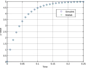
Open the files openloop_DE_A.slx and openloop_driver.m. These files generate both a Matlab and a Simulink simulation of the unit step response for the discrete-time transfer function

1 1 1 0. ( ) 1 0.8 8 p z z G z z      

In the time domain this corresponds to the difference equation y n( )0.8 (y n 1) u n( 1)

2 .

Figure 1. Open loop response of the system.

2) Now open up openloop_DE_A.slx (double click on it). It should look like Figure 2. We will be going through a number of the elements in this model so you can see how everything works.

Figure 2. openloop_DE_A.slx

0 0.05 0.1 0.15 0.2 0.25

0 0.5 1 1.5 2 2.5 3 3.5 4 4.5 5

Time

y

v

a

lu

e

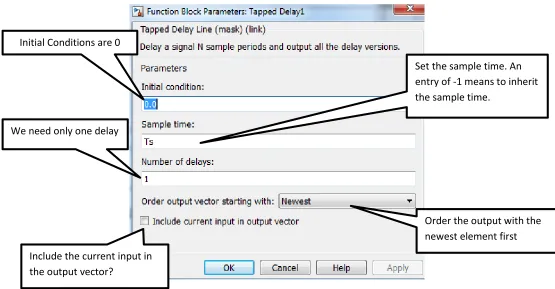
3 Starting at the left of the model (Figure 2), the input goes into a Delay Block (Tapped Delay 1). If you click on this delay block you will get the parameter block shown in Figure 3. This figure also shows what many of the parameters mean.

Figure 3. Parameter block for first delay, with explanations.

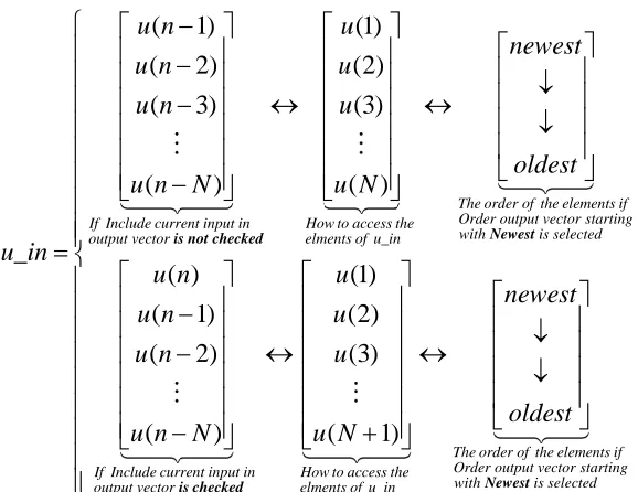
The output of this block is a scalar or a column vector. Figure 4 indicates the structure of this vector and how to access elements of the vector. This is important to remember!

Initial Conditions are 0

Set the sample time. An entry of -1 means to inherit the sample time.

We need only one delay

Order the output with the newest element first Include the current input in

4 _

( 1) (1)

( 2) (2)

( 3) (3)

( ) ( )

_

The order o If Include current input in How to access the

output vector elments of u in

u n u

newest

u n u

u n u

oldest

u n N u N

u in         _          _                          _       

 is not checked

( ) (1)

( 1) (2)

( 2) (3)

( ) ( 1)

f the elements if Order output vector starting with is selected

If Include current input in How to access t output vector

u n u

u n u

u n u

u n N u N

     _                      _   _      Newest

is checked _

The order of the elements if Order output vector starting he

with is selected elments of u in

newest oldest            _{ }  _{ }  _  _   _{  }  _{ }  _{ }    Newest

Figure 4. Output structure of a delay block. In the top row the current input is not included in the output. For both rows we assume there are N delays and the elements are in the newest first order. The middle vectors show how to access elements of the vector.

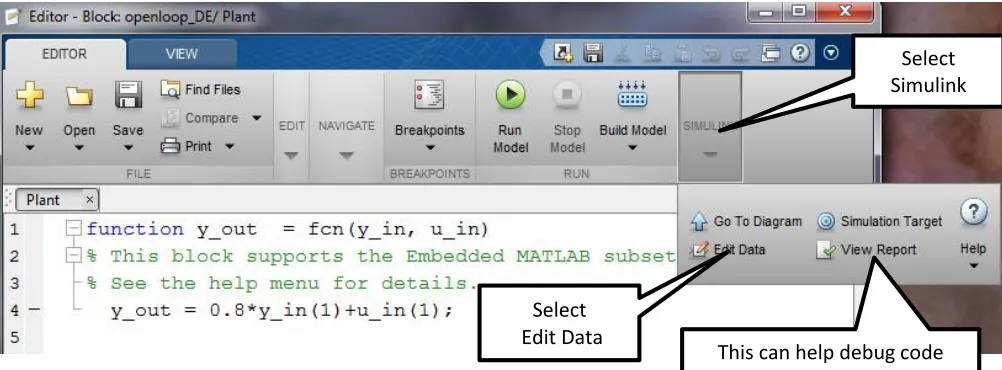
Now click on the plant (the large block in the center of Figure 2) and you will get the innocent looking piece of code for implementing a discrete-time transfer function shown in Figure 5. There are two things “passed” to this function: y_in, and u_in.

Figure 5. Code inside the plant block for implementing a discrete-time transfer function.

5 Figure 6. Accessing the “passed” items to this block via the Edit Data icon.

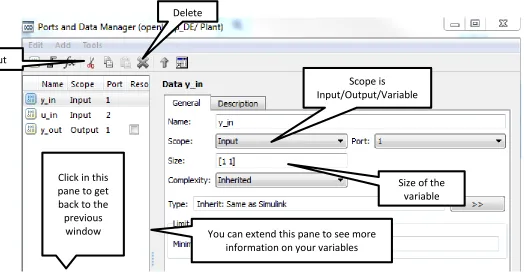
Once you click on the Edit Data icon, you will get a window like that shown in Figure 7.

Figure 7. Modifying variables and parameters

If you select one of the variables (such as y_in), you will get a figure like that in Figure 8. Click in the left-half plane to get back to the previous window.

Select Simulink

Select Edit Data

Variable Name

Input/Output Port

Add Data (new variables or parameters)

6 Figure 8. Information on simulation variables.

Referring to Figures 7 and 8,

 If the scope is a parameter, then you should not expect it to change as the simulation is running. If the scope is an input or output, then you should expect it to change as the simulation is

running, such as y_in, r_in, and y_out.

 The port indicates the order in which the variable will appear in the left (input) or right (output) side of the block. For this simulation, the port of y_in is one and the port of u_in is two, and this is reflected in how they are placed on the left of the plant block (See Figure 2).

 Most likely you will be changing the Size of the variables more than anything else.

 Add Data allows you to add new variables and parameters.

Scope is Input/Output/Variable

Size of the variable Cut

Delete

Click in this pane to get back to the previous

7 Part B

Copy openloop_DE_A.slx to openloop_DE_B.slx (save Openloop_DE_A as openloop_DE_B) and modify code as needed to determine the step response of the discrete-time plant

1 1 1 0.2 ( ) 1 0.8 p z z z G     

Assume a sampling interval of 0.1 seconds and run the simulation for 3 seconds. You should start by writing out the appropriate difference equation. You will then have to

 modify the first delay bock,

 modify the plant block so the size of u_in is correct (make a column vector)

 modify the code inside the plan block

 change the transfer function in the Matlab driver file

 change the Simulink file the Matlab driver file invokes

If Matlab complains that there is an error in the Simulink model, it is often useful to click on the Simulink block in question and then select View Report (See Figure 6.). This will often help find the errors.

When you run the Matlab driver file you should get a plot like that shown in Figure 9. Include your plot in your memo.

Figure 9. Step response for

1 1 1 0.2 ( ) 1 0.8 p z z z G     

0 0.5 1 1.5 2 2.5 3

8 Part C

Copy openloop_DE_B.slx to openloop_DE_C.slx and modify the code (both Matlab and Simulink) as needed to determine the step response of the discrete-time plant

1 2 1 2 0 0.2 ( ) 1 0. .1 0 6 1 . p z G z z z z    _    

Assume a sampling interval of 0.1 seconds and run the simulation for 2 seconds. You should start by writing the difference equation in the time domain. You will need to change both of the delay blocks and the plant block (both the code and the dimensions of the signals.) You should get a plot like that shown in Figure 10. Include your plot in your memo.

Figure 10. Step response for

1 2 1 2 0 0.2 ( ) 1 0. .1 0 6 1 . p z G z z z z    _    

0 0.2 0.4 0.6 0.8 1 1.2 1.4 1.6 1.8 2

9 Part D

Now we want to implement a controller in addition to our plant. As with our plants, it is easiest to get everything correct if you first write out a difference equation, and then figure out what you need in the delays and sizes of variables.

Copy your Simulink file openloop_DE_A.slx to closedloop_DE_A.slx. Your plant for part A should already be modelled correctly, and now we want to implement the integral controller ( ) 0.04

1

c

G z z



 . We also want a delay between the output and the input, so H z( )z1 (this is a simple delay). To implement the controller, again write out the difference equation in the time domain, and then modify

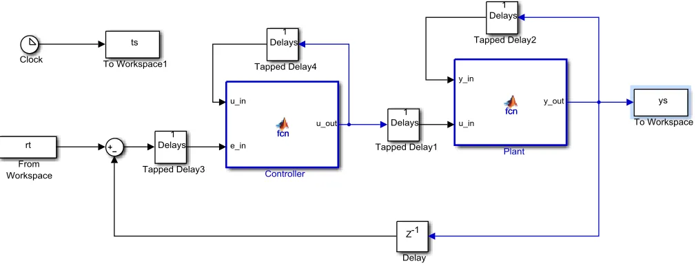
closedloop_DE_A.slx so it looks something like that in Figure 11. Note that the input is now rt, not ut, and the input and output variables in the controller have different names than for the plant. It is

probably easiest to copy your plant and then make it a controller.

Figure 11. Closed loop system for plant A.

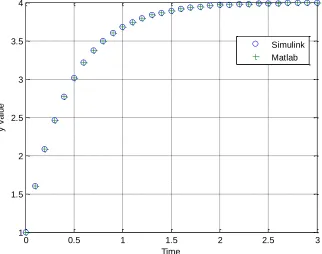
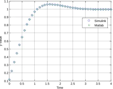
10 Figure 12. Result of Matlab and Simulink simulations for system A with an integral controller.

Part E

Copy your Simulink file openloop_DE_B.slx to closedloop_DE_B.slx. Your plant for part B should already be modelled correctly, and now we want to implement the proportional +integral controller

0.115(z 0.547) ( )

1

c z

z

G  

 . We also want a delay between the output and the input, so

1 ( )

H z z (this is a simple delay). You may also want to copy parts of your model from closedloop_DE_A.slx. To

implement the controller, again write out the difference equation in the time domain, and then modify closedloop_DE_B.slx so it again looks something like that in Figure 11 (though the delays may be different). After you have modified this file and the Matlab driver file (with a sampling interval of 0.1 sec), your results should look like those in Figure 13. Include your plot in your memo.

0 1 2 3 4 5 6 7 8

0 0.2 0.4 0.6 0.8 1 1.2 1.4

Time

y

v

a

lu

e _Simulink

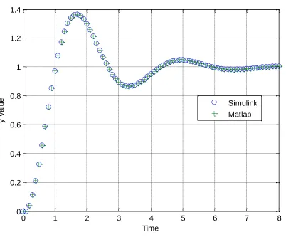
11 Figure 13. Result of Matlab and Simulink simulations for system B with a

proportional plus integral controller.

Part F

Copy your Simulink file openloop_DE_C.slx to closedloop_DE_C.slx. Your plant for part C should already be modelled correctly, and now we want to implement the proportional +integral+derivative controller

2

1.0631( 0.316 0.199) ( )

( 1) c

z z

G z

z z

 



 . We also want a delay between the output and the input,

so H z( )z1 (this is a simple delay). To implement the controller, again write out the difference equation in the time domain, and then modify closedloop_DE_C.slx so it again looks something like that in Figure 11 (though the delays may be different). After you have modified this file and the Matlab driver file (with a sampling interval of 0.1 sec), your results should look like those in Figure 14. Include your plot in your memo.

0 0.5 1 1.5 2 2.5 3 3.5 4

0.1 0.2 0.3 0.4 0.5 0.6 0.7 0.8 0.9 1 1.1

Time

y

v

a

lu

e

12 Figure 14. Result of Matlab and Simulink simulations for system C with a

proportional plus integral plus derivative controller.

Background: While PID controllers are very versatile, they have a number of drawbacks. One of the

major drawbacks is that for a unit step input, the control effort u t( ) can be infinite at the initial time.

This is referred to as a set-point kick. There are two commonly used configurations of PID controls schemes that utilize a different structure, the PI-D and the I-PD controllers. These are a bit more difficult to model using Matlab’s sisotool, but it can be done and we get to explore more of sisotool.

The PD controller avoids the set-point kick by putting the derivative in the feedback path, while the I-PD controller avoids the set-point kick by placing both the derivative and proportional terms in the feedback path. In the remainder of this lab we will implement both types of controllers using the embedded system toolbox.

0 0.5 1 1.5 2 2.5

0 0.1 0.2 0.3 0.4 0.5 0.6 0.7 0.8 0.9 1

Time

y

v

a

lu

e

13

Both of these controllers have the general form shown in Figure 15, where you can see we actually have two controllers in our system now.

For a PI-D controller we have

1 1

( ) ( )

( )

1 1 1 1

p i p

i i

p p

k k z k

k k z K z a

z k k

z C

z z z

             1 2 ( 1)

( ) (1 ) d

d

k z

C z k z

z

 

  

while for the I-PD controller we have

1( ) 1

1 1

i i

k k z

z

z z

C  _ 

 

1 2

( )

1) ( )

( ) (1 ) k d( p d d

p d p

k k z k

k z k z b

C z k k z

z z z

    

      

For both of these controllers, the closed loop transfer function is





1 ( ) ( ) ( ) ( )

p o

p

G

G

F z C z G z z

H z z C z C z



 

Now we are going to use sisotool to help initially design these controllers which you will then implement in the embedded system toolbox. You should go through the following example before going on to your own design.

When you start sisotool you need to click on the appropriate Control Architecture to get the proper configuration. Be sure that sisotool uses negative feedback for both loops (see Figures 16 and 17). Once you have the appropriate control architecture click OK (see Fgure 17). The you need to select Loop Configuration to set up the two loops (see Figures 16, 18, and 19.)

14

Figure 16. Changing the control architecture.

Click here to change the

control architecture

Click here to set up the Loop Configurations (See

15 Figure 17. This is the control architecture we want. Be sure that both S1 and S2 have a negative sign, then click OK.

In the block Open-loop configuration for: select Open Loop Output of C1 and select Open for Output of Block C2 (see Figure 18), then click OK.

In the block Open-loop configuration for: select Open Loop Output of C2 and select Open for Output of Block C1 (see Figure 19), then click OK.

Note that the above two steps are not absolutely necessary, but I find it a bit less confusing. The controllers in each window may not be exactly what you are expecting, but it is easier to visualize this way.

16 Figure 18. Open Loop Output of C1 Block.

17 Figure 20. The sisotool View window. We want to see the root locus plots for both Open Loop 1 and Open Loop 2.

For practice, let’s assume we have the plant from part C, ₂ 0.1 0 0.2 ( )

0.1 .6

p

G

z z z

z

 

  with a sampling

interval Ts = 0.1 seconds. When we import the plant andH z( )z1 (you may have to enter these in the Matlab workspace) we should get a design window that looks like that in Figure 21. Each root locus plot shows the plant with two identical proportional controllers.

If we implement a PI-D controller with ₁( 0.854( 0.7 4) 1

) 3

z z

C

z

 

 (left window)and 2

0.278(

(z) z 1)

C

z

 

18

19 Figure 22. Root lcous plots for a PI-D controller.

Figure 23. Step response (and control effort) for the PI-D controller in Figure 22.

-1 -0.5 0 0.5 1

-1 -0.8 -0.6 -0.4 -0.2 0 0.2 0.4 0.6 0.8 1

Root Locus Editor for Open Loop 2(OL2)

Real Axis

-1 -0.5 0 0.5 1

-1 -0.8 -0.6 -0.4 -0.2 0 0.2 0.4 0.6 0.8 1

Root Locus Editor for Open Loop 1(OL1)

Real Axis

Step Response

Time (seconds)

A

m

p

lit

u

d

e

0 0.5 1 1.5 2 2.5

20

If we implement an I-PD controller with ₁( ) 1.48 1

C z z

z



 (left window)and 2

0.15 0

) 8

( (z .2 )

C

z

z   (right

window) you should get a root locus plot like that shown in Figure 24, and a step response like that in Figure 25. (Note that the axis has been changed for both graphs in Figure 24 from what sisotool chose.)

Figure 24. Root lcous plots for an I-PD controller.

Figure 25. Step response (and control effort) for the I-PD controller in Figure 24.

-1 -0.5 0 0.5 1

-1 -0.8 -0.6 -0.4 -0.2 0 0.2 0.4 0.6 0.8 1

Root Locus Editor for Open Loop 2(OL2)

Real Axis

-1 -0.5 0 0.5 1

-1 -0.8 -0.6 -0.4 -0.2 0 0.2 0.4 0.6 0.8 1

Root Locus Editor for Open Loop 1(OL1)

Real Axis Step Response Time (seconds) A m p lit u d e

0 0.5 1 1.5 2 2.5 3 3.5

21 Part G You are now to implement the PI-D controller in above example using the embedded system

toolbox. The plant is ₂ 0.1

0 0.2 ( )

0.1 .6

p G z z z z  

  and the controllers are 1

0.854( 0.7 ( 4) 1 ) 3 z z C z  

 and

2

0.278(

(z) z 1)

C

z



 Note that we used the plant from system C so that file is probably the best place to

start. You also need to modify the Matlab driver code so that you can use Matlab to check your answers. You should name your Simulink file PI_D_C.slx. Your embedded system file should something like that in Figure 26, and if everything is working correctly you should get an output like that in Figure 27.

Include this figure (and an appropriate caption) in your memo.

Part H You are now to implement the I-PD controller in the previous example using the embedded

system toolbox. The plant is ₂ 0.1

0 0.2 ( )

0.1 .6

p G z z z z  

  and the controllers are 1

1.48 ( )

1

C z z

z



 and

2

0.15 0

) 8

( (z .2 )

C

z

z   Note that we used the plant from system C and the structure is nearly identical to that for part G, so that file is probably the best place to start (however you should rename your file to I_PD_C.slx.) You also need to modify the Matlab driver code so that you can use Matlab to check your answers. Tf everything is working correctly you should get an output like that in Figure 28. Include this figure (and an appropriate caption) in your memo.

22 Figure 27. Results for part G.

Figure 28. The results for part H.

0 0.5 1 1.5

0 0.2 0.4 0.6 0.8 1 1.2 1.4

Time

y

v

a

lu

e

Simulink Matlab

0 0.2 0.4 0.6 0.8 1 1.2 1.4 1.6 1.8 2

0 0.2 0.4 0.6 0.8 1 1.2 1.4

Time

y

v

a

lu

e

23 Part I For the plant ( ) ₂ 0.5

1

p

G

z z

z



  with a sampling interval Ts 0.1design and simulate (in both Matlab and using the embedded system toolbox) PI-D and I-PD controllers to meet the following specifications:

PO < 15%, Ts < 0.9seconds.