ECONOBOTICS – OPERATIONAL MODELS OF THE ENTERPRISES COMPETITIVENESS

(1)

ECONOBOTICS – OPERATIONAL MODELS OF THE ENTERPRISES COMPETITIVENESS

Ioana ARMAS, Ph.D.

^∗

Abstract. The competitiveness management is one of the most important and critical process in an enterprise, that has, as a main goal, the global quality implementation according to which the enterprise becomes a leader in its external environment, and has strong implications on the markets, society, and upon the natural environment,

Thus, in the context of the econobotic framework introduced and defined in [1] and specified in [2] the present paper will develop the fundamental specific operational models that will be used in the analysis and design of the enterprise’s evolution for global quality and competitiveness.

According to the TSE – space definition as the competitiveness space, the concepts and representations of the enterprise’s existence will be identified, and the models regarding competitiveness orientation and location, and actions will be developed.

The determined models represent the context for analysis and strategies design regarding the evolution of the enterprise in its complex external environment, in a manner that considers its behavior from the point of view of competitiveness and global quality.

Keywords: econobotics, competitiveness, enterprises evolution, competitiveness orientation, competitiveness location, econobotic actions.

1. Introduction

Considering the enterprise’s competitiveness goal as the global quality implementation according to the specific directions (see [3]), results that the competitiveness management will be considered and developed at the specific physical, biological, human, social, technical and economic econobotics reality levels [2].

In this context the existence and competitiveness position of the enterprise in the external and internal environments are of interest in establishing the strategies and actions of the management in a proactive manner, and in designing its functions, structures and interactions for short, medium and long terms. The corresponding decisions are supported by different models, mainly economic, and by simulations.

∗

Hyperion University, Bucharest, Romania [email protected]

(2)

The econobotic approach considers the enterprise as an econobotic system characterized by complexity, heterogeneity, and governed by synergistic relations and interactions that evolves in the TSE – space. From this point of view, the econobotic model of the competitiveness evolution for the enterprise will be developed as analysis and decisional support for the competitiveness management.

2. Concepts and models of the enterprise’s existence and competitiveness in the TSE – space

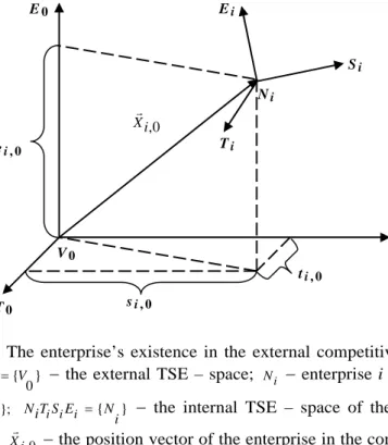
For the TSE – space context defined in [2] and assigned to the external environment, results that the enterprise’s existence is expressed by its internal TSE – space as in figure 1.

Figure 1. The enterprise’s existence in the external competitiveness space.

0 } 0 { 0 0

0 T S E V

V = − the external TSE – space; N

_i

− enterprise i in the TSE – space };

{V 0 { }

N i E S i T

N

_i _i _i

= − the internal TSE – space of the enterprise’s existence; X G _i _, ₀ − the position vector of the enterprise in the competitiveness space.

In the context of figure 1, the econobotic concepts and elements attached to the model of the enterprise’s existence are determined as following:

T

₀

S

₀

E

₀

V

₀

0 ,

X G i N

_i

T

_i

S

_i

E

_i

e

_{i , 0}

s

_{i , 0}

t

_{i , 0}

(3)

a) The position vector X G _i _, ₀

relative to { V

₀

} is determined by the column matrix of the homogeneous coordinates of the enterprise in the external TSE – space, { V

₀

}, as:

. ] 1 [

1 ]

[ _, ₀ _, ₀ _, ₀

0 ,

T i

i i i

i i

i t s e

e s t

X =

⎥ ⎥

⎦

⎤

⎢ ⎢

⎣

⎡

= (1)

b) The orientation of the internal TSE – space { N relative to the

_i

} external one { V

₀

} is determined by the orientation matrix expressed in homogeneous coordinates:

, 1 0 0 0

0 0 0

1 0

0 0

0 ) , cos(

) , cos(

0 ) , cos(

) , cos(

0 ) , cos(

) , cos(

] [

/ 3 / 2 / 1

0 0

0

0 0

0

0 0

0

0 ,

⎥ ⎥

⎦

⎤

⎢ ⎢

⎣

⎡

ε ε ε

σ σ σ

θ θ θ

=

⎥ ⎥

⎥

⎦

⎤

⎢ ⎢

⎢

⎣

⎡

= Ο

i i i

i i

i

i i

i

E T E S E E

E S S

S T

S

E T S

T T

T

(2)

where ( Λ

₀

, Γ

_i

) with Λ = T , S , E and Γ = T , S , E represent the orientation angles between two axis of { V

₀

} and respectively, { N

_i

}.

The ( Λ

₀

, Γ

_i

) angles with Λ = Γ represent technical, social, and economic orientations of the enterprise relative to the ones considered as reference in the external environment, and the ( Λ

₀

, Γ

_i

) angles with Λ ≠ Γ represent the corresponding influences upon the other dimensions of the internal TSE – space, { N

_i

}, relative to the external one, { V

₀

}.

c) The location of the enterprise in the external competitiveness space is determined by the competitiveness matrix [ C ]

_i_,₀

that integrates both the orientation of the internal TSE – space { N relative to the external one

_i

}

},

{ V

₀

and its position in { V

₀

}, as following:

(4)

. 1 0 0 0 ]

[

0 , / 3 / 2 / 1

0 ,

⎥ ⎥

⎦

⎤

⎢ ⎢

⎣

⎡

ε ε ε

σ σ σ

θ θ θ

=

i i i i

i

e

s t

C (3)

The [ C ]

_i_,₀

matrix represents how the enterprise’s competitiveness is perceived by the external environment.

Also, a [ C ]

₀_,_i

= [ C ]

⁻_i¹_,₀

matrix will represent how the competitiveness space is represented by the enterprise at its internal TSE – space level, and is determined according to (2) and (3) by the following relation:

=

⎥ ⎥

⎥

⎦

⎤

⎢ ⎢

⎢

⎣

⎡

=

1 0

0 0

) , cos(

] [

, 0 0 0

0

, 0 0 0

0

, 0 0 0

0 ,

i i

o i i

i

E T E S E E e

s E S S

S T

S

t E T S

T T

T C

1/ 1/ 1/ 1/ ,0 1/ ,0 1/ ,0

2 / 2 / 2 / 2/ ,0 2/ ,0 2/ ,0

3/ 3 / 3 / 3/ ,0 3/ ,0 3/ ,0

( )

( ) .

0 0 0 1

i i i i i i i i i

t s e

θ σ ε − θ ⋅ + σ ⋅ + ε ⋅

⎡ ⎤

⎢ ⎥

θ σ ε − θ ⋅ + σ ⋅ + ε ⋅

⎢ ⎥

= ⎢ ⎢ θ σ ε − θ ⋅ + σ ⋅ + ε ⋅ ⎥ ⎥

⎢ ⎥

⎣ ⎦

(4)

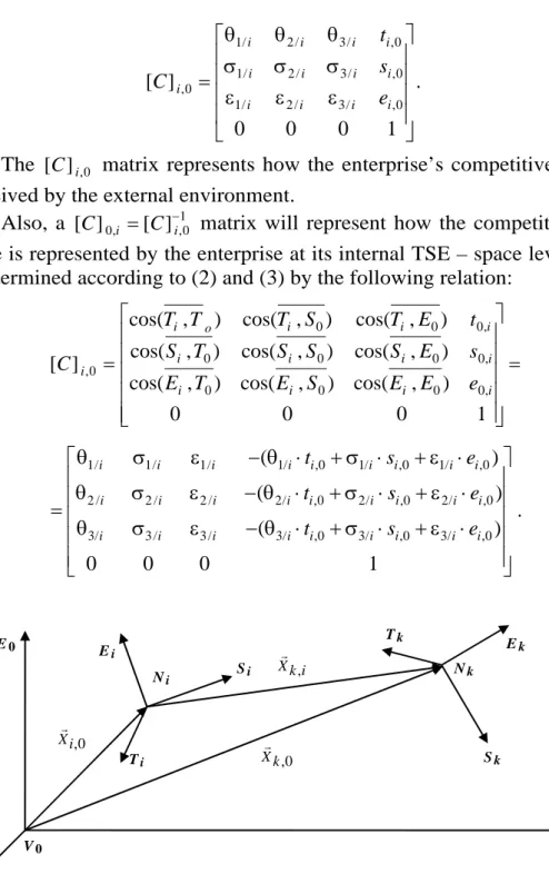
Figure 2. The competition configuration between the enterprises { i N } and { N

_k

}.

T

₀

S

₀

E

₀

V

₀

0 , X G i

N

_i

T

_i

S

_i

E

_i

N

_k

T

_k

S

_k

E

_k

0 , X G k

i

X , G k

(5)

The competition configuration between two enterprises is represented in figure 2 and is determined by the relative competitiveness location in the TSE – space:

, 1 0 0

0 ]

[

, , / 3 , / 2 , / 1

,

⎥ ⎥

⎦

⎤

⎢ ⎢

⎣

⎡

ε ε

ε

σ σ

σ

θ θ

θ

=

i k i k i k i k

i

k e

s t

C (5)

where θ _v _/ _k _, _i = cos( T _i , Γ _k ), σ _v _/ _k _, _i = cos( S _i , Γ _k ), ε _v _/ _k _, _i = cos( E _i , Γ _k ) for ,

3 , 2 ,

= 1

v and Γ

_k

= T

_k

, S

_k

, E

_k

determine the orientation of the enterprise }

{ N

_k

relative to { N

_i

}, and [ X ]

_k_,_i

= [ t

_k_,_i

s

_k_,_i

e

_k_,_i

1 ]

^T

is the position of }

{ N

_k

relative to { N

_i

}, expressed in homogeneous coordinates.

Applying relation (4), the competitiveness location of { N relative to

_i

} }

{ N

_k

will be determined as:

, 1 0 0

0 ]

[

, , / 3 , / 3 , / 3

, , / 2 , / 2 , / 2

, , / 1 , / 1 , / 1

,

⎥ ⎥

⎦

⎤

⎢ ⎢

⎣

⎡

ε σ

θ

ε σ

θ

ε σ

θ

=

k i i k i k i k

k

i e

s t

C (6)

with the position of N relative to

_i

{ N

_k

} expressed in normal coordinates for a 3-D space given by the position vector [ N _i ] _k = [ t _i _, _k s _i _, _k e _i _, _k ] ^T , where:

⎪ ⎩

⎪ ⎨

⎧

⋅ ε +

⋅ σ +

⋅ θ

−

=

⋅ ε +

⋅ σ +

⋅ θ

−

=

⋅ ε +

⋅ σ +

⋅ θ

−

=

).

(

) (

, , / 3 , , / 3 , , / 3 ,

, , / 2 , , / 2 , , / 2 ,

, , / 1 , , / 1 , , / 1 ,

i k i k i k i k i

k i k k

i

i k i k i k i k i

k i k k

i

i k i k i k i k i k i k k

i

e s

t e

e s

t s

e s

t t

The relative competitiveness locations [ C ]

_k_,_i

, [ C ]

_p_,_k

for three enterprises N _i , N _k , N _p are, composed in the [ C ]

_p_,_i

competitiveness location of { N _p } relative to { N

_i

}, determined with the relation:

k p i k i

p

C C

C ]

_,

[ ]

_,

[ ]

_,

[ = ⋅ . (7)

The ‘absolute’ competitiveness location of { N _p } in the universe (i.e., external environment) { V

₀

} is determined by:

i p i

p

C C

C ]

_,₀

[ ]

_,₀

[ ]

_,

[ = ⋅ . (8)

(6)

Relations (7) and (8) are generalized for any number of enterprises N

n

N

₁

,

₂

, ... , as following:

, ] [ ]

[ ...

] [ ] [ ] [

1

, 1 1

, 2

, 3 1 , 2 1

,

∏

⁻

= +

−

=

⋅

=

ⁿ

k

k k n

n

C C C C

C (9)

and respectively:

. ] [ ]

[ ...

] [ ] [ ] [ ] [ ] [ ] [

1

0

, 1 1

, 2

, 3 1 , 2 0 , 1 1

, 0 , 1 0

,

∏

⁻

= +

−

=

⋅

=

⋅

=

ⁿ

k

k k n

n n

n

C C C C C C C

C (10)

3. The action – oriented model of the enterprise

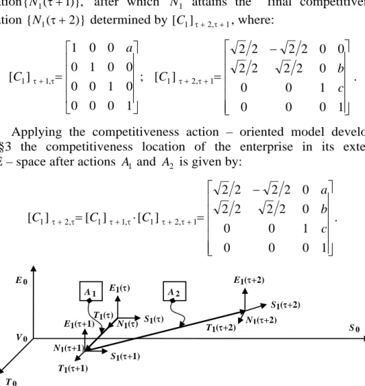
The objectives and decisions of the enterprise are integrated and expressed by its actions in the TSE – space. From this point of view, the following elementary actions are determined as in table 1, such that any evolution instance or trajectory is a composition of a number of successive elementary actions.

Table 1.

Elementary actions in the TSE – space.

1. Social – economic competitiveness orientation (SEO)

CPO – conventional positive orientation

⎥ ⎥

⎥

⎦

⎤

⎢ ⎢

⎢

⎣

⎡

α α

α

−

= α τ + τ

1 0 0 0

0 cos sin 0

0 sin cos

0 0 0 0 1 , ] 1 [ i C

2. Technical – economic competitiveness orientation (TEO)

⎥ ⎥

⎥

⎦

⎤

⎢ ⎢

⎢

⎣

⎡

β β

−

β β

τ = + τ

1 0 0 0

0 cos 0 sin

0 0 1 0

0 sin 0 cos ,

] 1 [ i C N

_i

( τ ) =

= N

_i

( τ + 1 )

S

_i

( τ ) =

= S

_i

( τ + 1 ) T

_i

( τ )

E

_i

( τ )

T ( τ + 1 ) E

_i

( τ + 1 )

β > 0 β > 0

CPO N

_i

( τ ) = N

_i

( τ + 1 )

T

_i

( τ ) = T

_i

( τ + 1 )

S

_i

( τ ) E

_i

( τ )

S

_i

( τ + 1 ) E

_i

( τ + 1 )

α > 0 α > 0

CPO

(7)

3. Technical – social competitiveness orientation (TSO)

CPO – conventional positive orientation

⎥ ⎥

⎥

⎦

⎤

⎢ ⎢

⎢

⎣

⎡

γ γ

γ

− γ τ =

+ τ

1 0 0 0

0 1 0 0

0 0 cos sin

0 0 sin cos ,

] 1 [ i C

4. Technical competitiveness (positive or negative) evolution (P/N-TE)

⎥ ⎥

⎥

⎦

⎤

⎢ ⎢

⎢

⎣

⎡

τ = + τ

1 0 0 0

0 1 0 0

0 0 1 0

0 0 1 , ] 1 [

a C i

5. Social competitiveness (positive or negative) evolution (P/N-SE)

⎥ ⎥

⎥

⎦

⎤

⎢ ⎢

⎢

⎣

⎡

τ = + τ

1 0 0 0

0 1 0 0

0 1 0

0 0 0 1 , ] 1

[ b

C i

6. Economic competitiveness (positive or negative) evolution (P/N-EE)

⎥ ⎥

⎥

⎦

⎤

⎢ ⎢

⎢

⎣

⎡

τ = + τ

1 0 0 0

1 0 0

0 0 1 0

0 0 0 1 , ] 1

[ C i c

N

_i

( τ )

E

_i

( τ ) = E

i

( τ + 1 )

S

_i

( τ ) T

_i

( τ )

S

_i

( τ + 1 ) T

_i

( τ + 1 )

c > 0 N

_i

( τ + 1 ) N

_i

( τ )

T

_i

( τ )

E

_i

( τ ) E

_i

( τ + 1 ) b > 0

N

_i

( τ + 1 )

T

_i

( τ + 1 )

S

_i

( τ ) = S

_i

( τ + 1 ) N

_i

( τ )

T

_i

( τ ) = T

_i

( τ + 1 )

S

_i

( τ ) E

_i

( τ )

S

_i

( τ + 1 ) E

_i

( τ + 1 )

a > 0

N

_i

( τ + 1 )

N

_i

( τ ) = N

i

( τ + 1 ) E

_i

( τ ) = E

_i

( τ + 1 )

S

_i

( τ )

T

_i

( τ )

S

_i

( τ + 1 )

T

_i

( τ + 1 )

γ > 0

CPO

(8)

7. General competitiveness orientation (GEO)

⎢ ⎢

⎣

⎡

τ + τ τ + τ τ + τ

ε ε

ε

σ σ

σ

θ θ

θ τ = + τ

0 0

0 ,

] 1 [

, 1 / 3 , 1 / 2 , 1 / 1

C i

8. General competitiveness (positive or negative) evolution (P/N-GE)

⎥ ⎥

⎥

⎦

⎤

⎢ ⎢

⎢

⎣

⎡

τ = + τ

1 0 0 0

1 0 0

0 1 0

0 0 1 , ] 1

[ c

b a C i

9. General competitiveness orientation and evolution (GCOE)

⎢ ⎢

⎣

⎡

τ + τ τ + τ τ + τ

ε ε

ε

σ σ

σ

θ θ

θ τ = + τ

0 0

0 ,

] 1 [

, 1 / 3 , 1 / 2 , 1 / 1

C i

Any action is specified as A

_τ₊₁

= ( c

_τ₊₁

, w

_τ₊₁

, f

_τ₊₁

) , where c

_τ₊₁

represents the initial conditions given by the last location of the enterprise,

)}, (

{ N

_i

τ w

_τ₊₁

− the contents of the action (i.e., orientation, evolution, or different combinations), f

_τ₊₁

− the effect of the action given by [ C _i ] _τ ₊ ₁ _, _τ that determines the new location { N

_i

( τ + 1 )}. In this context, an action A _τ ₊ ₁ is a transition from { N

_i

( τ )} to { N

_i

( τ + 1 )}, and is represented by:

)}

1 ( { )}

(

{ N _i τ ⎯ ⎯ → ^A ^τ ⎯ ⁺ ⎯ ¹ N _i τ + . (11)

N

_i

( τ )

T

_i

( τ ) S

_i

( τ )

S

_i

( τ + 1 ) E

_i

( τ + 1 )

[ a , b , c ]

^T

N

_i

( τ + 1 ) T

_i

( τ + 1 ) E

_i

( τ )

N

_i

( τ )

T

_i

( τ ) S

_i

( τ )

S

_i

( τ + 1 ) E

_i

( τ + 1 )

[ a , b , c ]

^T

N

_i

( τ + 1 ) T

_i

( τ + 1 ) E

_i

( τ )

N

_i

( τ ) = N

_i

( τ + 1 )

T

_i

( τ + 1 )

S

_i

( τ ) E

_i

( τ )

S

_i

( τ + 1 ) E

_i

( τ + 1 )

T

_i

( τ )

(9)

A succession of actions defined as:

)}

( { )}

1 (

{

...

)}

2 ( { )}

1 ( { )}

( {

1 1 2

n N n

N

N N

N

i i

i

A n A n

A A

+ τ

⎯

⎯ →

⎯

− + τ

⎯

⎯ →

⎯

→

→ +

τ

⎯

⎯ →

⎯ + τ

⎯

⎯ →

⎯ τ

+ τ

− + τ

+ + τ

τ

(12) will be represented by a composed action

, ...

)

( n A

₁

A

₂

A

_n

A τ → τ + =

_τ₊

D

_τ₊

D D

_τ₊

(13)

and its global effect relative to the initial internal TSE – space of the enterprise, { N

_i

( τ )}, will be given by the matrix:

, ]

[ ]

[ ...

] [ ] [ ]

[

1

0

, 1 1

, 1

, 2 ,

1

,

∏

⁻

= τ+ + τ+

− + τ + τ +

τ + τ τ + τ τ

+

τ

= ⋅ ⋅ ⋅ =

ⁿ

k

k k i n

n i i

i n

i

C C C C

C (14)

where [ C

_i

]

_τ₊_k₊₁_,_τ₊_k

, k = 0 , n − 1 is the effect matrix of action A

_{τ k}₊ ₊₁

. Matrix [ C _i ] _τ ₊ _n _, _τ will determine the final competitiveness location of the enterprise after the n actions, relative to its initial location, { N

_i

( τ )}, and applying relation (10), the final location of the enterprise in the competitiveness space { V

₀

} will be given by:

, ] [ ] [ ]

[ ] [ ]

[ C _i _τ ₊ _n _, ₀ = C _i _τ _, ₀ ⋅ C _i _τ ₊ _n _, _τ = C _i _i _, ₀ ⋅ C _i _τ ₊ _n _, _τ (15) where [ C

_i

]

_τ_,₀

= [ C ]

_i_,₀

represents the initial location of the enterprise

} { )}

(

{ N

_i

τ = N

_i

relative to { V

₀

}. .

Relations (12) ÷ (15) and table 1 define the competitiveness action – oriented model of the enterprise, that supports the analysis and design of the competitiveness strategies in attaining a goal expressed as a location in the TSE – space, by determining the corresponding and necessary actions.

4. Analysis case for an enterprise in the TSE – space

In figure 3, the successive effect locations of an enterprise N are

₁

considered after the following actions: A − positive technical evolution

₁

with a units advance relative to its initial competitiveness location { N

₁

( τ )},

after which N attains the competitiveness location

₁

{ N

₁

( τ + 1 )} determined

by [C

₁

]

_τ₊₁_,_τ

, A − general evolution with

₂

[ 0 b c ]

^T

and technical – social

competitiveness orientation with γ = 45

^D

relative to its competitiveness

(10)

location { N

₁

( τ + 1 )}, after which N attains the final competitiveness

₁

location { N

₁

( τ + 2 )} determined by [ C

₁

]

_τ₊₂_,_τ₊₁

, where:

. 1 0 0 0

1 0 0

0 2 2 2 2

0 0 2 2 2

2 ]

[

; 1 0 0 0

0 1 0 0

0 0 1 0

0 0 1 ]

[ ₁ ₁ _, ₁ ₂ _, ₁

⎥ ⎥

⎥

⎦

⎤

⎢ ⎢

⎢

⎣

⎡ −

=

⎥ ⎥

⎦

⎤

⎢ ⎢

⎣

⎡

= _τ ₊ _τ ₊

τ +

τ c

C b a

C

Applying the competitiveness action – oriented model developed in §3 the competitiveness location of the enterprise in its external TSE – space after actions A and

₁

A is given by:

₂

. 1 0 0 0

1 0 0

0 2 2 2 2

0 2 2 2

2 ]

[ ]

[ ₁ ₂ _, ₁ ₁ _, ₁ ₂ _, ₁

⎥ ⎥

⎥

⎦

⎤

⎢ ⎢

⎢

⎣

⎡ −

=

⋅

= _τ ₊ _τ _τ ₊ _τ ₊

τ +

τ c

b a C

C C

Figure 3. The competitiveness locations of the enterprise {N 1 } after actions A ₁ and A 2 .

5. Conclusions

The presented paper extends the field of econobotics defined and introduced in [1, 2] by developing the concepts and models of the enterprise’s existence and competitiveness in the TSE – space. In this context the behavior of the enterprise is expressed by its actions in the competitiveness space and, accordingly, the competitiveness action – oriented model is developed.

The results create the framework for analysis and design of the

T

₀

E

₀

V

₀

E

₁

(τ)

T

₁

(τ) S

₁

(τ) N

₁

(τ)

S

₁

(τ+1) E

₁

(τ+1)

T

₁

(τ+1)

T

₁

(τ+2)

S

₁

(τ+2) E

₁

(τ+2)

N

₁

(τ+1)

N

₁

(τ+2)

S

₀

A

₁

A

₂

(11)

competitiveness oriented manner. From this point of view, an analysis case has been developed as an example of the action – oriented model direct application.

R E F E R E N C E S

[1] I. Armas, Econobotics – A New Framework for the Enterprises Development, Hyperion International Journal of Econophysiscs and New Economy 2015, Volume 8, Issue 2, pp. 203-303.

[2] I. Armas, Econobotics Reality Levels in the Enterprises Evolution Analysis, Hyperion International Journal of Econophysiscs and New Economy 2016, Volume 9, Issue 1, pp. 107-114.

[3] I. Armas, Mechatronic Products and Services (in Romanian), Editura AGIR, Bucharest, 2009.

[4] I. Armas, Design for Mechatronics and Robotics (in Romanian), Editura AGIR, Bucharest, 2011.

[5] I. Armas, Social Robotics. Innovative Models and Consciousness (in Romanian),

Editura AGIR, Bucharest, 2016.

ECONOBOTICS – OPERATIONAL MODELS OF THE ENTERPRISES COMPETITIVENESS