For human society both soil and water are highly important natural resources that need to be care-fully treated and every care has to be taken to sustain them. They are very closely related – at
the fundamental level sediment, consisting of solid soil particles eroded from a specific source, is transported by a medium – water. Soil and aquatic environments are thus linked together.
Sediment Load and Suspended Sediment Concentration
Prediction
Martin Bečvář
Institute of Water and environment, Cranfield University at Silsoe, england, United
Kingdom, and Department of Irrigation, Drainage and Landscape engineering, Faculty
of Civil engineering, Czech Technical University in Prague, Prague, Czech Republic
Abstract: Sediment is a natural component of riverine environments and its presence in river systems is essential. However, in many ways and many places river systems and the landscape have been strongly affected by human activities which have destroyed naturally balanced sediment supply and sediment transport within catchments. As a consequence a number of severe environmental problems and failures have been identified, in particular the link between sediments and chemicals is crucial and has become a subject of major scientific interest. Sediment load and sediment concentration are therefore highly important variables that may play a key role in environ-ment quality assessenviron-ment and help to evaluate the extent of potential adverse impacts. This paper introduces a methodology to predict sediment loads and suspended sediment concentrations (SSC) in large European river basins. The methodology was developed within an MSc research study that was conducted in order to improve sediment modelling in the GREAT-ER point source pollution river modelling package. Currently GREAT-ER uses suspended sediment concentration of 15 mg/l for all rivers in Europe which is an obvious oversimplification. The basic principle of the methodology to predict sediment concentration is to estimate annual sediment load at the point of interest and the amount of water that transports it. The amount of transported material is then redistributed in that corresponding water volume (using the flow characteristic) which determines sediment concentrations. Across the continent, 44 river basins belonging to major European rivers were investigated. Sus-pended sediment concentration data were collected from various European basins in order to obtain observed sediment yields. These were then compared against the traditional empiric sediment yield estimators. Three good approaches for sediment yield prediction were introduced based on the comparison. The three approaches were applied to predict annual sediment yields which were consequently translated into suspended sediment concentrations. SSC were predicted at 47 locations widely distributed around Europe. The verification of the methodology was carried out using data from the Czech Republic. Observed SSC were compared against the predicted ones which validated the methodology for SSC prediction.
Via sediment, representing the connection, all components of soil may be transferred into aquatic environments. The system of sediment supply and sediment transport was naturally balanced until human society, causing pressure on both river systems and landscape, interrupted these links. Such interruption has resulted in various severe environmental problems. Soil fertility is gradu-ally decreasing due to an excessive level of soil erosion; aquatic environments suffer from high sediment inputs, typically rich in nutrients and chemicals, which affects water quality, aquatic habitat, engineering structures, navigation and, generally, the potential to use water. Effects on water quality and related issues are probably the most significantly apparent and debated problems caused by sediment. Sediment yield and sediment concentration are therefore highly sought after elements of environmental information, providing a possibility to assess the magnitude of running processes in catchments and their potential impacts on the environment. However, the understanding of sediment concentrations, sediment supply and transfer is still not complete. Predicting sediment concentration is particularly difficult and is still challenging the scientific community as there is a high degree of uncertainty involved, and the controlling processes are rarely predictable.
This research aims to develop a methodology to predict sediment yield (SY) and suspended sediment concentrations (SSC) for a randomly selected point on a river within a catchment. A requirement for such a method was originally envisaged together with an intention to improve sediment modelling in the GREAT-ER river pack-age. GREAT-ER (Feijtel et al. 1997) is a steady state river model which is used to assess the im-pact of chemicals on the aquatic environment. It has been developed for the European Chemicals Industry Council (CEFIC) in anticipation of new EC legislation on chemicals. Currently GREAT-ER uses just one sediment concentration of 15 mg/l for all rivers in Europe. This is obviously oversimpli-fied and needed to be improved. An MSc research study (Bečvář 2005) was undertaken in order to establish a solid base for the development of a suitable methodology. The specific objectives of this research were therefore as follows:
− to investigate and collate available spatial and
temporal pan-European data sets;
− to develop or select suitable European soil erosion
and sediment yield estimation approaches;
− to test the performance of the traditional
exist-ing sediment yield estimators against observed sediment yield data;
− to establish good approaches as a result of the
testing;
− to use the best approaches for predicting
sedi-ment yields where observed records are not available; and
− to translate predicted sediment yields into
sedi-ment concentrations where observed are not available.
Having such objectives, the main focus of the literature review was soil erosion, sediment sup-ply, sediment sources and sediment transport processes. Special emphasis was paid to sediment yield estimation methods that were particularly important for the method development.
The material transported by a river stream must have a source somewhere in the catchment further upstream. Rarely is it just one source. Normally there are a number of sediment sources identi-fied. However, generally, sediment sources can be divided into two groups:
(1) Sediment which is generated by a river itself as a consequence of natural- or human-initiated bed-forming processes. River channel changes, both vertical and cross profile, act on flood plains continually to modify the river‘s shape to adjust-ing its dimensions in order to comply with dis-charges. Remobilization of stored sediment, bank erosion and pool and riffle creation, for example, all generate sediment from the natural content of rivers. However, thanks to human activities these processes may be disturbed and accelerated to an excessive level, which can lead to negative impacts.
(2) Sediment which is supplied to channels from surrounding areas. In this case there are several factors which are crucial in terms of erosion risks, namely relief character, soil and climatic properties, land cover and land use in particular. Processes of soil erosion on agricultural land and the con-sequences of construction and mining activities are examples of significant potential sources of sediment. In fact, any location in which the soil is not strong enough to resist the erosive forces placed upon it, and where there are suitable con-ditions for transport of eroded material, can be labelled a sediment source
relevance. As previously stated there were two sediment sources identified to be of major im-portance for SSC prediction – soil erosion within the catchment and river bank erosion. These were consequently further investigated and available methods for their assessment on a European scale were examined.
In terms of soil erosion a number of projects have attempted to provide complex information about soil erosion risks at national, European and international level. Usually a map of soil erosion in Europe was produced as an outcome. Typical examples are the PESERA approach (Kirkby et al. 2003), the INRA approach (Le Bissonnais et al. 2002), the USLE approach (Van der Knijff et al. 2000), the GLASOD approach (Van Lynden 1994), the CORINE approach (CORINE 1992) and the RIVM approach (RIVM 1992). These approaches were carried out on different bases. Therefore criteria were formed in order to select an appropriate approach to be further applied for SSC prediction. Some of the main drawbacks of particular approaches were discussed by Grimm et al. (2002). The criteria for rejecting an approach were, for example, too low spatial resolution, lim-ited spatial availability of soil erosion informa-tion over large parts of the continent or a lack of soil erosion information in GIS format. The most suitable approach was thus identified to be the PESERA approach. The PESERA soil erosion approach became a fundamental data source that was relevant for testing SY and sediment delivery ratio (SDR) approaches and later also for sediment concentrations predictions.
The second source of material relevant for SSC prediction was bank erosion. Although there are methods for assessing bank erosion (Environment agency 1999) they are difficult to apply over such large areas and miscellaneous environments as investigated here. Therefore the only considered source of material was soil erosion. Certainly the original intention was to try to evaluate all the potential sediment sources, but the lack of as-sessment methods or essential data, meant it was only possible to deal with soil erosion. However soil erosion information alone does not indicate how much material is actively transported – sedi-ment yield does. Sedisedi-ment yield, together with the amount of water available to transport the material, also primarily determines sediment concentrations. Sediment yields can be generally estimated using either process based models or the
traditional empiric models. Process based models that take into account laws of mass and energy conservation are not usually applicable over such large study areas. The traditional sediment yield estimation methods use either direct computa-tion from catchment parameters or a sediment delivery ratio (SDR). Sediment yield can be then calculated as follows:
SY = a × X + b × Y + c × Z
where:
X, Y, Z – catchment parameters a, b, c – regression coefficients or the second possibility: SY = SOIL EROSION × SDR
Such SDR methods are also predominantly based on defining statistically significant links between observed yields and catchment parameters. The most commonly used catchment parameters are the area, relief, length (or relief-length ratio) and slope of the catchment. A number of SDR compu-tation methods can be found in literature. Some authors have also related sediment yield to river network density (Roehl 1962), land cover (Wil-liams 1977), runoff (Dendy & Bolton 1976) or soil properties (Walling 1983). In the literature review sixteen SY estimation approaches (either direct computation or using the SDR) were re-viewed (Bečvář 2005). It is presumed that these approaches produce considerably different results depending on selected parameters and conditions under which they have been developed. The in-tention was to use all of them and compare them against observed values to see which ones seem to be performing well. Nonetheless, essential data sources were either missing or were not accurate enough to evaluate all the parameters required for sediment yield or SDR estimation. Therefore only seven approaches were used and tested (Maner 1958; Anonym 1971; Williams & Berndt 1972; McPherson 1975; Renfro 1975; Vanoni 1975).
plays a role in high flows. Obviously the type of behaviour is determined by the amount of sediment supplied. The system of sediment concentrations is often hysteretic. Hysteretic loops can be observed during flood events when SSC are plotted against discharge. Although a wide range of sediment con-centrations can be seen in any particular flow it can be concluded that it is still true that the majority of material is transported in high flows.
The issues reviewed above provided sufficient background and understanding in order to deter-mine a solid knowledge base for the SSC prediction method development. In the following section the key points of the methodology development are addressed and the current state of sediment concentration prediction is described.
MAteriAL And MethodS
The basic principle of the methodology to predict sediment concentration is to estimate annual sedi-ment load at the point of interest and the amount of water that transports it. The amount of transported material is then redistributed in that corresponding water volume (using the flow characteristic) which determines sediment concentrations.
Hence:
SC (mg/l) = annually transported material (mg) annual water volume (l) (i)
In order to obtain the first part of the equation, sediment yields methods were tested. Suspended sediment and flow data were collected from various European catchments, namely the Rhine, Mosel, Rhone, Jucar, Ebro, Elbe, Morava and Oder. Having obtained sediment concentrations and discharge data, real sediment yields were calculated using
the equation (i). Consequently sediment yield estimators (listed in previous chapter) were used to obtain calculated sediment yields at the same location where SSC data exist. This provided a great opportunity to compare both observed and calculated values. The comparison showed that results obtained using the USDA SCS (1971) SDR method correlate best with the observed yields. Therefore this method was selected to be used for sediment yield estimation. In addition, further analyses on monitored SSC were carried out in or-der to introduce two new relationships. Observed sediment yields were related directly to the rate of soil erosion (calculated using the PESERA ap-proach) found in catchment delineated above the point of interest. This is shown in Figure 1.
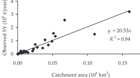
[image:4.595.82.529.598.729.2] [image:4.595.303.531.599.727.2]It was discovered that sediment yield is equal to approximately one fifth of soil erosion. Another link was identified between observed sediment yield and the area of the catchment. This shows Figure 2.
These three methods were then introduced as those most suitable for sediment yield prediction and were used to calculate annually transported material – the first variable in the equation (i). The second parameter in the equation is the amount of water in which the material is transported. Since sediment yields were calculated as annual, annual water volume at the point of interest was required. That could have been easily done using the flow data, and annual mean sediment concen-tration could have been calculated. However this research aimed to go a little bit further than that. The intention was not to be restricted to just one value of SSC but to provide information about the variability of sediment concentrations in different flows. In order to do so, sediment concentration behaviour in different flows had to be determined.
y = 0.22x R2 = 0.86
0 1 2 3 4
0 2 4 6 8 10 12 14
Soil erosion – PESERA (106 t/year)
O
bs
er
ve
d
SY
(1
0
6 t/
yea
r)
y = 20.53x R2 = 0.84
0 1 2 3 4
0.00 0.05 0.10 0.15
Catchment area (106 km2)
O
bs
er
ve
d
SY
(1
0
6 t/
yea
r)
[image:4.595.62.297.603.726.2]Figure 2. A link between observed sediment yields and corresponding catchment areas
For that purpose the flow exceedance curve was used. However instead of plotting the discharge sediment concentration occurring in that particular discharge were plotted. In doing so, the relation-ship between flow exceedance and SSC could be observed. Figure 3 shows an example from the river Rhine at Koblenz in Germany.
It is quite obvious that a law can be established here. SSC behaviour can be divided into two parts. In the first part up to Q30 sediment concentrations remain relatively constant whereas in the second part, in flows higher than Q30 they change logarith-mically. The SSC prediction was then also divided
into two parts according to that law. Of course, sediment yield and water volume as parameters to be utilised in the equation (i) had to be estimated separately for those two parts. By carrying out further analyses using the available SSC data it was found that flows of up to Q30 accounted for just 14% of total annually transported load, and thus in higher flows the remaining 86% is transported. Figure 4 shows the principle of the water volume estimation. A sum of areas over the whole data sample divided by a number of observation years determines the annual amount of water volume in flows higher than Q30.
0 80 160 240 320 400
0 20 40 60 80 100
Flow exceeded for %
SS
C
(m
g/l
[image:5.595.66.327.81.236.2])
Figure 3. Sediment concentrations plotted using the flow exceedance
¦³
³
³
³
³
n i n t n t t t i t i t t t dt t f dt t f dt t f dt t f dt t f Q 1 ) ( ) 1 ( ) 4 ( ) 3 ( ) 1 ( ) ( ) 2 ( ) 1 ( 300 . .
TOTAL dt t f Q Q n i
¦³
1 100 0 100 30 TOTAL TOTALMEAN ANNUAL WATER VOLUME Q1–30 = TOTAL Q0–30/no. YEARS (ii) Similarly the water volume in flows up to Q30 can be determined:
[image:5.595.91.514.397.745.2]MEAN ANNUAL WATER VOLUME Q30–100 = TOTAL Q30–100/no. YEARS (iii)
Figure 4. Water volume calculation for 30% flow exceedance Time D is ch arg e (m 3/s ) 2000 1800 1600 1400 1200 1000 800 600 400 200 0
0
200
400
600
800
1 000
1 200
1 400
1 600
1 800
2 000
Time
D
isc
ha
rg
e
(m
3
/s
)
exceeded for 30 %
f(t)
Exceeded for 30% f(t)
It can be written as follows (f(t) is a function describing discharge in time):
Having estimated the water volume it was then fairly straightforward to calculate SSC occurring in flows up to Q30 using the equation. For flows higher than Q30, a function describing the data had to be determined. The monitored SSC data from various European basins were analysed. The function was produced consequently:
SSC(Q30–0) = –47.16 ln(x) + 183.66
where:
x – percentage of flow exceedance
At this point the methodology seemed to be consistent and ready to be applied. However dur-ing the predictions some major imperfections were identified. Figure 5 illustrates the critical shortcoming.
ent curve, showing the variations of sediment concentrations in a certain flow level, discreet values of SSC were aimed. Figure 6 shows this modification.
It is fairly self-explanatory – for each ten per-cent of flow exceedance a representative SSC was estimated. The numbers reflect how much of the annual sediment yield is transported in this par-ticular part of the flow.
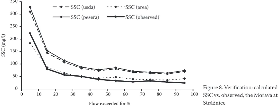
The methodology was verified using data from the Czech Republic. The Czech Hydrometeorological Institute provided high quality data (daily SSC) at three locations: the Elbe at Děčín, the Morava at Strážnice and the Oder at Bohumín. Predicted SSCs were compared with the observed ones. The following Figures 7–9 show the comparisons.
reSuLtS And diSCuSSion
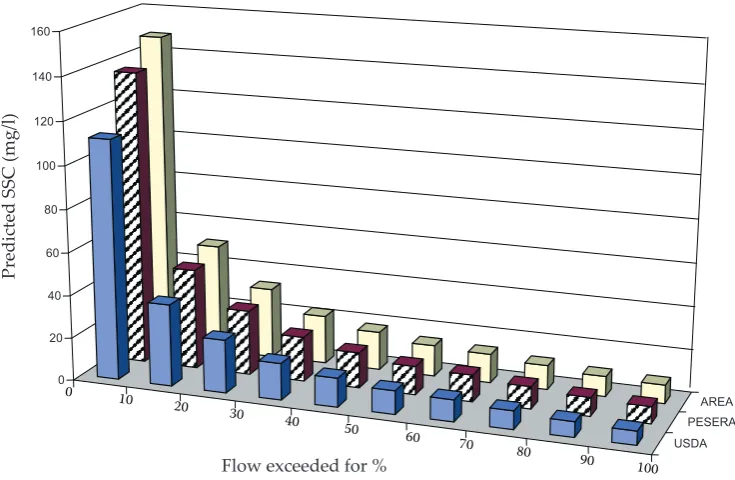
The result of this research was a successful de-velopment of a methodology to predict sediment concentration. The method was applied and used for SSC prediction at 47 locations. Figure 10 shows an example of predicted sediment concentration using the three sediment yield estimators.
Although the verification proved the methodol-ogy performs well, there are several issues that need to be further discussed. The study area includes 44 basins that cover almost the entire continent. Therefore, as well as natural boundaries (such as the catchement ones) there are also political boundaries which make any modelling particu-larly difficult. Especially important is the fact that some parameters and typically involved processes have an inherently high level of uncertainty, such as sediment yields and sediment concentrations. Different environmental policies and land man-agement practices may significantly influence Figure 5. Shortcomings in the methodology
In some cases a step in SSC progress appeared or sediment concentrations were of negative values. In order to eliminate this, the methodology was slightly modified. Instead of producing a
coher-62.9%
14.3% 7.7%
4.6% 3.2% 2.3% 1.9% 1.4% 1.0% 0.7%
Flow exceeded for %
M
at
er
ia
l t
o
be
tr
an
sp
or
te
d
%
o
f a
nn
ua
l
0 10 20 30 40 50 60 70 80 90 100
Flow exceeded for % Figure 6. Modification of the methodology
-100 0 100 200 300 400
0 20 40 60 80 1
Flow exceeded for %
SS
C
(m
g/
l)
[image:6.595.64.278.353.480.2]Figure 7. Verification: calculated SSC vs. observed, the Elbe at Děčín
Figure 8. Verification: calculated SSC vs. observed, the Morava at Strážnice
sediment patterns even within one catchment. Nevertheless even this would not be a major is-sue if good quality data existed. Data availability was perhaps the main limiting factor in the meth-odology development. The fact that suspended sediment concentration data were not collected from all the catchments was to a certain extent limiting to the development of a methodology, and moreover even the collected ones were not of the same quality. The data were from different sources with temporal resolution varying from daily to monthly (or even longer) sampling periods. In terms of SSC predictions the main weakness lies in the fact that it does not take local conditions into account. Local conditions may significantly influence sediment concentration; however, no available method could be applied over such large areas as investigated here in order to take them
into account. Therefore actual suspended sediment concentration may differ in orders of magnitude (reservoir trap efficiency or additional sediment sources may play a key role). The error on SSC prediction when all the other sediment sources were omitted also needs to be further investigated. Nonetheless the values obtained by applying the methodology can be considered for use in the GREAT-ER river package. The mean suspended sediment concentration extracted from all the avail-able monitored SSC data was 23 mg/l. The mean from all the predicted ones was 50 mg/l whereas GREAT-ER uses just 15 mg/l. That means that the amounts of chemicals, associated in GREAT-ER with the particular sediment concentration, may be underestimated.
At the moment however, the sediment concen-trations must still be treated as provisional ones 0
40 80 120 160 200
0-10 10-20 20-30 30-40 40-50 50-60 60-70 70-80 80-90 90-100 Flow exceeded for %
SS
C
(m
g/
l)
SSC (usda) SSC (area)
SSC (pesera) SSC (observed)
0 50 100 150 200 250 300 350
0-10 10-20 20-30 30-40 40-50 50-60 60-70 70-80 80-90 90-100Flow exceeded for %
SS
C
(m
g/
l)
SSC (usda) SSC (area)
SSC (pesera) SSC (observed)
0 10 20 30 40 50 60 70 80 90 100
Flow exceeded for %
[image:7.595.65.532.577.758.2]due to the relatively crude estimations used during the prediction. The methodology currently has its shortcomings and drawbacks; nevertheless another study with an objective to eliminate them is cur-rently underway. A PhD study entitled “Study of erosion and sediment transport in the Elbe catch-ment in the Czech Republic” aims to focus on the main shortcomings of the methodology. The scale of the forthcoming study is much bigger and good quality data have been obtained so far. Thus it pro-vides a great opportunity to continue this research and further develop and refine the methodology. It is expected then that other relevant knowledge
Figure 10. An example of predicted sediment concentration using the three sediment yield estimators
will be gained that will support the understanding of the behaviour of sediment concentrations and improve their prediction. Sediment concentra-tion is a critical parameter with highly indicative value that provides an opportunity to evaluate the seriousness of potential environmental impacts. Its prediction is therefore desirable.
references
Anonym (1971): National Engineering Handbook, Sec-tion 3: SedimentaSec-tion, Chapter 6: Sediment sources, yields, and delivery ratios. USDA, Washington.
USDA PESERA
AREA 0
20 40 60 80 100 120 140 160
Pr
ed
ic
te
d
SS
C
(m
g/l
)
Flow exceeded for %
Danube@Regensburg
0 10
20 30
40 50
60 70
[image:8.595.105.473.489.729.2]80 90 100
Figure 9. Verification: calcu-lated SSC vs. observed, the Oder at Bohumín
0 50 100 150 200 250
0-10 10-20 20-30 30-40 40-50 50-60 60-70 70-80 80-90 90-100 Flow exceeded for %
SS
C
(m
g/
l)
SSC (usda) SSC (area)
SSC (pesera) SSC (observed)
Bečvář M. (2005): Estimating typical sediment concent-ration probability density functions for European rivers. [M.Sc. Thesis.] Cranfield University, Silsoe, England. CORINE (1992): Soil Erosion Risk and Important Land
Resources in the Southern Regions of the European Community. Luxembourg: EUR 13233.
Dendy F.E., Bolton G.C. (1976): Sediment yield-runoff drainage area relationships in the United States. Journal of Soil and Water Conservation, 31: 264–266.
Environment agency (1999): Waterway Bank Protection: A Guide to Erosion Assessment and Management. Environment Agency, Bristol.
Feijtel T., Boeije G., Matthies M., Young A., Mor-ris G., Gandolfi C., Hansen B., Fox K., Holt M., Koch V., Schroder R., Cassani G., Schowanek D., Rosenblom J., Niessen H. (1997): Development of a geography-referenced regional exposure assessment tool for European rivers – GREAT-ER. Chemosphere, 34: 2351–2373.
Grimm M., Jones R., Montanarella L. (2002): Soil Erosion Risk in Europe. Office for Official Publications of the European Communities, Luxembourg.
Kirkby M.J., Jones R.J.A., Irvine B., Gobin A. (2003): Pan-European Soil Erosion Risk Assessment. Office for Official Publications of the European Communities, Luxembourg.
Le Bissonnais Y., Thorette J., Bardet C., Daroussin J. (2002): L’erosion hydrique du sols en France. Technical Report INRA et IFEN.
Maner S.B. (1958): Factors Influencing Sediment Delivery Rates in the Red Hills Physiographic Area. In: Transac-tions of the American Geophysical Union: 669–675.
McPherson H.J. (1975): Sediment yields from intermedi-ate sized stream basins in Southern Alberta. Journal of Hydrology, 25: 243–257.
Renfro G.W. (1975): Use of erosion equations and sedi-ment delivery ratios for predicting sedisedi-ment yield. In: Present and Prospective Technology for Predicting Sediment Yield and Sources. USDA, Washington. RIVM (1992): The Environment in Europe: A Global
Perspective. RIVM, Bilthoven.
Roehl J.E. (1962): Sediment Source Areas, Delivery Ratios and Influencing Morphological Factors. IAHS, 52: 202–213.
Van der Knijff J.M., Jones R.J.A., Montanarella L. (2000): Soil Erosion Risk Assessment in Europe. EUR 19044 EN.
Van Lynden G.W.J. (1994): The European Soil Resource: Current Status of Soil Degradation in Europe: Causes, Impacts and Need for Action. ISRIC, Strasbourg. Vanoni V.A. (1975): Sedimentation Engineering. In:
Manuals and Reports on Engineering Practices, ASCE, New York.
Walling D.E. (1983): The sediment delivery problem. Journal of Hydrology, 65: 209–237.
Williams J.R. (1977): Sediment Delivery Ratios Deter-mined with Sediment and Runoff Models. In: Erosion and Solid Matter Transport in Inland Waters. IAHS, 122: 168–179.
Williams J.R., Berndt H.D. (1972): Sediment yield com-puted with universal equation. Journal of Hydraulics Division ASCE, 98: 2087–2098.
Received for publication December 14, 2005 Accepted January 9, 2006
Corresponding author: