An improved photometric stereo through distance
estimation and light vector optimization from diffused
maxima region
Jahanzeb Ahmad1
, Jiuai Sun, Lyndon Smith, Melvyn Smith
Centre for Machine Vision, Bristol Robotics Laboratory, University of the West of England, Bristol, UK
Abstract
Although photometric stereo offers an attractive technique for acquiring
3D data using low-cost equipment, inherent limitations in the methodology
have served to limit its practical application, particularly in measurement or
metrology tasks. Here we address this issue. Traditional Photometric Stereo
assumes that lighting directions at every pixel are the same, which is not
usually the case in real applications, and especially where the size of object
being observed is comparable to the working distance. Such imperfections
of the illumination may make the subsequent reconstruction procedures used
to obtain the 3D shape of the scene prone to low frequency geometric
distor-tion and systematic error (bias). Also, the 3D reconstrucdistor-tion of the object
results in a geometric shape with an unknown scale. To overcome these
problems a novel method of estimating the distance of the object from the
camera is developed, which employs photometric stereo images without using
Email addresses: [email protected](Jahanzeb Ahmad),
[email protected](Jiuai Sun), [email protected](Lyndon Smith),
other additional imaging modality. The method firstly identifies Lambertian
diffused maxima region to calculate the object distance from the camera,
from which the corrected per-pixel light vector is able to be derived and the
absolute dimensions of the object can be subsequently estimated. We also
propose a new calibration process to allow a dynamic(as an object moves in
the field of view) calculation of light vectors for each pixel with little
addi-tional computation cost. Experiments performed on synthetic as well as real
data demonstrates that the proposed approach offers improved performance,
achieving a reduction in the estimated surface normal error of up to 45% as
well as mean height error of reconstructed surface of up to 6 mm. In
addi-tion, when compared to traditional photometric stereo, the proposed method
reduces the mean angular and height error so that it is low, constant and
independent of the position of the object placement within a normal working
range.
Keywords: Photometric Stereo, Light Vector Calculation, Distance
Estimation.
1. Introduction
1
Traditional Photometric Stereo (PS) is used to recover the surface shape
2
of an object or scene by using several images taken from the same view
3
point but under different controlled lighting conditions [1, 2]. It was initially
4
introduced by Woodham in 1980 [3]. PS has been extensively used in many
5
applications especially for estimating high density local surface normals in
6
the fields of computer vision and computer graphics. It has been used for
7
3D modelling [4], facial expression capturing [5, 6]. It has also been used for
medical applications [7, 8] and in face recognition security systems [9]. Most
9
of these applications require high accuracy reconstructed surfaces. So it is
10
critical to estimate high accuracy surface normals in order to get accurate
11
subsequent surface reconstruction from their integration. As we will show
12
in the following experiment setup, 2-3 degree error in surface normal can
13
produce up to 6 mm error in the height of reconstructed surface.
14
Current state-of-the-art systems normally assume that light sources are
15
at an infinite distance from the scene so that a homogeneous and parallel
16
incident light condition can be formed; and then the PS problem becomes
17
solvable through a group of linear equations. In reality it is not always
possi-18
ble to produce parallel(collimated) incident light, especially when the object
19
size is comparable in magnitude to the light separation and or the distance
20
of object from light source is relatively small. Any underestimation or
mis-21
alignment of the illumination may produce some error during recovery of the
22
surface normal. For example, a 1% uncertainty in the intensity estimation
23
will cause a 0.5-3.5 degree deviation in the calculated surface normal for a
24
typical three-light source photometric stereo setup [10]. Uncertainty in the
25
calibration process can also lead to systemic errors when recovering surface
26
normals and in the 3D recovered surface [11, 12].
27
Furthermore PS gives no information concerning the absolute distance of
28
the object from the camera. Other imaging modalities are normally required
29
for obtaining such range data, for example laser triangulation or stereo vision
30
techniques have been combined with the PS approach [13–17]. A dense
(per-31
pixel) surface reconstruction of a smooth and texture-less object proves to be
32
a challenging task for many range detection imaging approaches, since they
can only provide sparse surface data. In order to recover the range data at
34
pixel resolution, we may alternatively make use of some information about
35
the object surface itself such as convexity and smoothness.
36
In this paper we present a novel method to allow us to calculate the
37
distance of an object based on the same photometric stereo imaging setup,
38
i.e. one camera and four lights, without a requirement for any additional
39
hardware, but with little extra computation processing cost. The object’s
40
distance from the camera is estimated by finding small patches on the object
41
surface whose normal is pointing towards light source. This small patch is
42
also called the diffused maxima region (DMR) and has been recently [18] used
43
for solving the problem of the generalized bas-relief ambiguity (GBR) [19].
44
The estimated distance is then used to calculate the light vectors at every
45
image pixel, thereby minimizing the error associated with the assumption
46
of a collimated light source. This approach enables the photometric stereo
47
method to effectively work with real light sources, on Lambertian surfaces
48
that have at least one patch with normal vectors pointing directly towards
49
the light source, in reality this is a reasonable assumption.
50
To the best of our knowledge we are the first to use the DMR in this
51
way, i.e. to enhance the PS method by reducing the well know problem of
52
distortion in the recovered 3D surface by improving the light vector direction
53
estimation and adding range data by using the convexity and smoothness of
54
real objects and without using other additional imaging modalities. Paper is
55
organized as following, in next section we will discuss related work after that
56
photometric stereo technique is discussed. In section 4 proposed method is
57
discussed followed by experiments and results in section 5. Finally in section
6 paper is concluded.
59
2. Related Work
60
The common low cost approach to produce collimated light is to use
61
convex lenses or concave mirrors; but even in these cases, only a narrow
62
parallel light beam with similar physical size to that of the lens or mirror can
63
be obtained. To produce a collimated light source for a larger scene area,
64
a possible solution is to develop a custom optical system with an array of
65
specially aligned individual light units. Unfortunately this results in a high
66
hardware and setup cost [20]. Another practical solution is to set the light
67
sources far away from the object[21] , so that the light can be approximated
68
as a distant radiation point source. This strategy may help to provide evenly
69
distributed radiance across the object surface, but it sacrifices the majority
70
of the illumination intensity, and correspondingly decreases the signal/noise
71
ratio of the whole system. In addition, such a distant lighting setup usually
72
means a large impractical working space is required. So this approach is
73
only suitable for those light sources able to produce high levels of energy and
74
those applications where a large redundant space is available. In terms of
75
the availability and flexibility of current commercial illumination, the distant
76
illumination solution is often not an optimal choice.
77
A nearby light source model has been considered as an alternative by Kim
78
[22] and Iwahori [23] to reduce the photometric stereo problem to find a local
79
depth solution using a single non-linear equation. By distributed the light
80
sources symmetrically in a plane perpendicular to camera optical axis, they
81
of initial values for the optimisation process and limitations in the speed for
83
solving non-linear equation are the main problems with this method.
84
A moving point light source based solution has been proposed by Clark
85
[24] termed “Active Photometric Stereo”. By moving a point light along a
86
known path close to the object surface a linear solution can be formulated to
87
solve the photometric stereo problem. However, the range of motion of light
88
must be closely controlled in order to guarantee the efficiency of the solution.
89
Kozera and Noakes introduced an iterative 2D Leap-Frog algorithm able
90
to solve the noisy and non-distant illumination issue for three light-source
91
photometric stereo [25]. Because distributed illuminators are commercially
92
available, Smith et al. approximated two symmetrically distributed nearby
93
point sources as one virtual distant point light source for their dynamic
pho-94
tometric stereo method [26]. Unfortunately, none of these methods lend
95
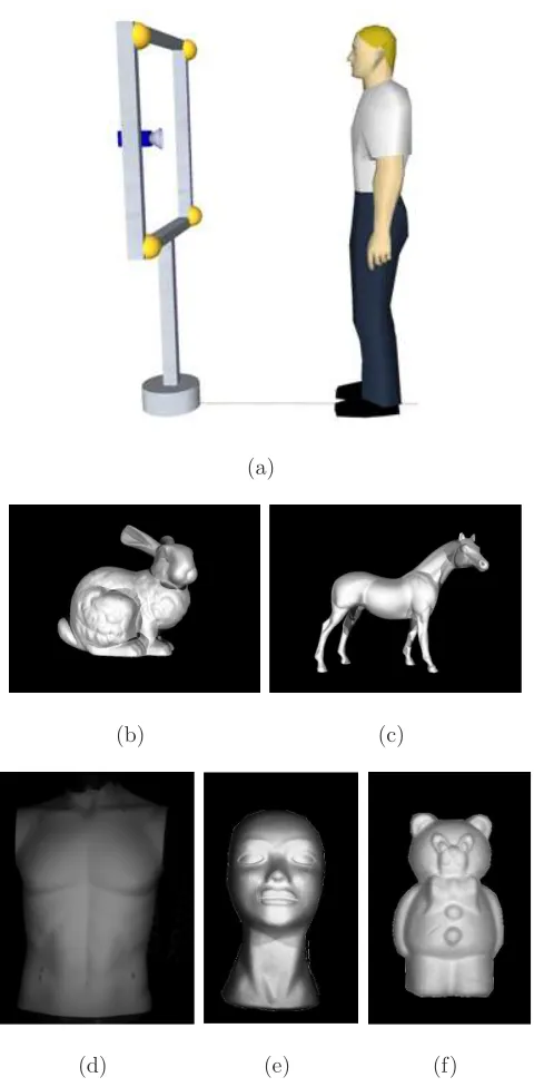
themselves to a generalized approach.
96
Varnavas et al. [27] implemented parallel CUDA based architecture and
97
computed light vectors at each pixel by manually placing shiny sphere at the
98
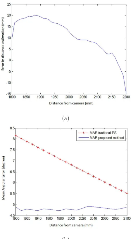
four corners of the field of view and assuming a flat plane at that distance,
99
so that a changing light direction was taken into account. However in
prac-100
tice the whole surface of the object is not flat and is not necessarily at the
101
same distance from the light source, especially when the size of the object is
102
comparable to the distance of the light source.
103
3. Photometric Stereo
104
According to the Lambertian reflectance model the intensity I of light
105
reflected from an object’s surface is dependent on the surface albedo ρ and
the cosine of the angle of the incident light as described in Equation 1. The
107
cosine of the incident angle can also be referred as dot product of the unit
108
vector of the surface normal −→N and the unit vector of light source direction
109
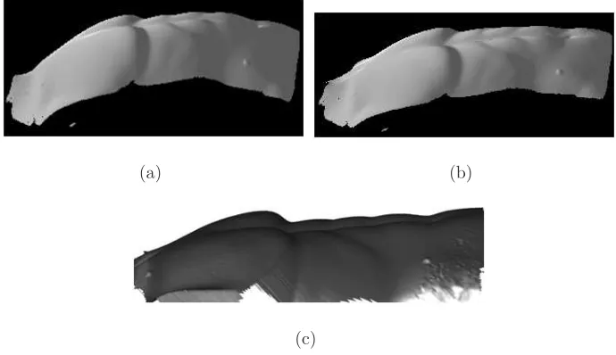
− →
L, as shown in Equation 2 .
110
I =ρcos(φi) (1)
I =ρ(−→L .−→N) (2)
When more than two images (four images are used in the following work)
111
from same view point are available under different lighting conditions, we
112
have a linear set of Equation 1 and 2 and this can be represented in vector
113
form as shown in Equation 3.
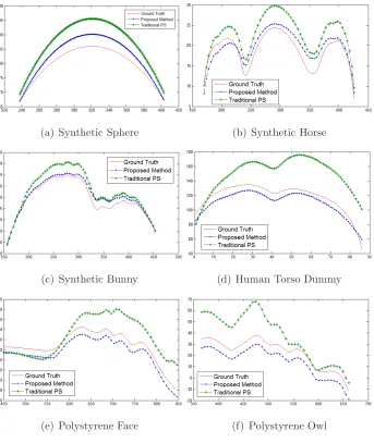
114
− →
I(x, y) = ρ(x, y)[L]−→N(x, y) (3)
− →
I is the vector formed by the four pixels ((I1
(x, y), I2
(x, y), I3
(x, y),
115
I4
(x, y))T from four images, [L] is the matrix composed by the light
vec-116
tors (−L→1;−L→2; −L→3;−L→4). Where, 1, 2, 3 and 4 is the number with respect to the
117
individual light source direction. [L] is not a square and so not invertible, but
118
the least square method can be used to compute Pseudo-Inverse and local
119
surface gradients p(x, y) and q(x, y), and the local surface normal N(x, y)
120
can be calculated from the Pseudo-Inverse using Equations 4,5 and 6 where
121
−→
M(x, y) = (m1(x, y), m2(x, y), m3(x, y)).
122
−→
p(x, y) = m1(x, y)
m3(x, y)
, q(x, y) = m2(x, y)
m3(x, y)
(5)
N(x, y) = p p(x, y), q(x, y),1
p(x, y)2
+q(x, y)2
+ 1 (6)
ρ(x, y) =
q
m2
1(x, y) +m 2
2(x, y) +m 2
3(x, y) (7)
4. Proposed Method
123
By estimating the distance of the object from the camera we can improve
124
the accuracy of the surface normals by calculating the light vector of every
125
pixel based on its distance from the camera and light source. The proposed
126
method is summarised in Pseudo code in Table 1. It is divided into three
127
parts: “Light source position estimation”, “Object distance estimation” and
128
“Per pixel light direction calculation”. Light source position estimation is
129
required only once during the rig calibration process.
130
4.1. Light source position estimation
131
The general assumption that the light vector is the same at every point
132
(pixel) is mostly not true in practice, so subsequently we use triangulation
133
and the intersection of at least two light vectors (calculated at different
posi-134
tions) to determine the true position of a light in a world coordinate system
135
at the optical centre as shown in Figure 1. A specular sphere is used to
calcu-136
late the light vectors at several (we take two as example) different locations
137
in the imaging area. The intersection of these light vectors is taken as the
138
position of the light in the real world coordinate system. The position of
Table 1: Pseudo code of proposed method.
1. Light Source Position Estimation.
1.1. Place a specular sphere in Field of view.
1.2. Calculate Light vector using equation 8.
1.3. Calculate position of highlight point in world coordinates using equation 19.
1.4. Repeat steps 1.1 to 1.3 by placing the sphere in another location.
1.5. Once two light vectors and two highlight positions for same light has been calculated using the
above steps, the position of light can be calculated using equation 11.
1.6. Repeat steps 1.1 to 1.5 for all light sources to calculate light positions.
1.7. Calculate light vectors of all lights by placing the sphere in the centre of field of view by using
equation 8. These light vectors will be called pseudo light vectors.
2. Object distance estimation.
2.1. Capture a sequence of images of the object.
2.2. Calculate surface normals by using pseudo light vectors and equation 6. Resultant normals are
called pseudo normals.
2.3. Calculate diffused maximum region by using equation 20.
2.4. Create a vector from centre of diffused maximum region to centre of lens as shown in Figure 3(a).
2.5. Now using origin of lens, pseudo light vector, position of light and vector created in step 2.4 we
can calculate distance of object by using the same intersection equations as used in step 1.5.
2.6. Repeat steps 2.2 to 2.4 for every light source and take average of all estimated distance values for
final estimated value.
3. Per pixel light direction calculation.
3.1. Draw an imaginary plan at the estimated distance.
light 1 is calculated by finding the intersection point of light vectors −L→11 and
140
−→
L12 as shown in Figure 1. −→
L11 is the light vector calculated at a sphere surface
141
position p1
1 by placing the sphere at one random location and
−→
L1
2 is the light
142
vector calculated at a sphere surface position p1
2 by placing the sphere at
an-143
other random location in the imaging area. To calculate −L→11 and −→
L12 Equation
144
8 is used.
145
− →
L = 2(−→n .−→d)−→n −−→d (8)
Where−→d is reflection direction taken as (0,0,1),−→n is unit surface normal
146
at point p1 1 or p
1
2, −→n = (nx, ny, nz), nx = px− cx, ny = py − cy and
147
nz =
q
(r2 −n2
x−n 2
y), (cx, cy) and (px, py) are the pixel coordinates of the
148
sphere centre and the highlight on the sphere respectively, and r is the radius
149
of sphere in the image plane.
[image:10.595.176.435.420.618.2]150
Figure 1: Calibration setup for light position calculation and initial (Pseudo) light vector
The intersection of−L→11 and −→
L12 can be calculated using equations 9, 10 and
151
11 [28]
152
Lp11 =p 1 1+
(−L→1 2×(p
1 1−p
1 2)).(
−→ L1 1× −→ L1 2)
(−L→11× −→
L12).( −→
L11× −→
L12)
!
∗−L→11 (9)
Lp1 2 =p
1 2+
(−L→1 1×(p
1 1−p
1 2)).(
−→ L1 1× −→ L1 2)
(−L→11× −→
L12).( −→
L11× −→
L12)
! ∗−L→1
2 (10)
Lp1 = Lp
1 1 +Lp
1 2
2 (11)
E =|Lp11 −Lp 1
2| (12)
Lp1
is the 3D position of light 1 in the world coordinate system. Lp1
1 is
153
the point on vector −L→11 closest to −→
L12, Lp 1
2 is the point on vector
−→
L12 closest
154
to −L→11, E is the distance between these two points - which can be used to
155
measure the accuracy of the calculation. If E is zero then both light vectors
156
intersect. However, due to error in estimating the light vector, the position
157
of the highlight or sphere centre E is not always zero or close to zero. So we
158
use a threshold to establish when the estimated light position is not accurate.
159
In this case the sphere can be positioned in additional places to improve the
160
accuracy.
161
To calculate the position of light using the above method we need the
162
position of at least two highlights on the sphere surface. These highlights
163
can be calculated by first calculating the centre of the sphere. As the actual
164
size of the sphere, focal length of the camera and physical pixel size of camera
sensor are known, we can find the position of the centre of the sphere in the
166
world coordinate system.
167
c(X, Y, Z) = [−x
fx
Z,−y fy
Z, Z] (13)
Z = f ocalLength∗sphereActualRadius
pixelLength∗sphereP ixelRadius (14)
WhereZ is the distance of sphere centre from camera in the z direction,fx
168
and fy are the focal length in pixels in xand y direction. Once the centre of
169
spherecis known, the surface normal −→n at pointp(highlight pixel position)
170
can be used to calculate p from equation 15.
171
p(X, Y, Z) =c(X, Y, Z) +k∗n(X, Y, Z) (15)
k is a constant required to calculate p. As p lies on the surface of the
172
sphere |p−c| should be equal to the sphere radius and by using value of p
173
from equation 15 we can solve the value of k from the following equations.
174
|c+k−→n −c|=sphereActualRadius (16)
|−→n|= 1 (17)
k =sphereActualRadius (18)
Once the value ofkis calculated, it can be used in equation 15 to calculate
175
the position of the highlight on the sphere surface in real world coordinates;
176
as shown in equation 19.
p(X, Y, Z) =c(X, Y, Z) +sphereActualRadius∗ −→n (19)
4.2. Object Distance Estimation
178
The object distance from the camera is calculated by using the Diffused
179
Maxima Region (DMR), which is calculated by taking the absolute of the
180
dot product between the pseudo light vector and pseudo surface normal, and
181
then applying a threshold; as shown in equation 20. During experimentation
182
we have found that for most cases the threshold is greater then or equal to
183
0.9.
184
DM Ri =| − →
N .−→Li|>0.9 (20) −
→
Li is a pseudo light vector for light i and−→N is the pseudo surface normal
185
at each pixel. The pseudo light vector−→Li is calculated during the calibration
186
process by placing the sphere at the centre of the field of view, it is assumed
187
to be same for every pixel. The centre of the DM R gives us the point
188
where the surface normal and the light vector are approximately aligned.
189
Many DM R(s) can exist on the surface of an object but the region with
190
maximum pixel area is considered to be the best choice. Lights are arranged
191
in a square arrangement as shown in Figure 4(a) and the dot product of the
192
light vectors with surface normals are shown in Figure 2. Higher value of dot
193
product means it is more close to diffused maxima. Figure 2 shows the four
194
selected DM R centres plotted on a height map of a synthetic sphere and a
195
real human dummy torso.
(a)
(b)
(c) (d)
Figure 2: (a) and (b) dot product of image with its light vectors. Diffused maxima regions
are in highlighted in dark red colour. (c) and (d) Diffused Maxima Regions centres are
[image:14.595.120.497.123.513.2](a) (b)
Figure 3: (a) Depth calculation using DMR and intersection of vector Ov and L1. (b)
Light vector calculation on each point of object surface.
Once the DM R centre is identified in the image plane, a vector −→Ov can
197
be created from the DM R centre to the centre of the lens O, as shown in
198
Figure 3(a). O is also the origin of the world coordinate system. Now by
199
using origin O, position of light LP, light vector −L→1
and vector −→Ov, we can
200
determine the intersection point of these two vectors in world coordinates by
201
using equations 9, 10 and 11. The average of the Zcoordinate of these points
202
of intersection is the estimated distance of the object from the camera.
203
4.3. Per pixel light direction calculation
204
Once the distance of the object is known from the camera, an imaginary
205
plane parallel to the image plane is created. The pseudo height of the object
206
is then defined relative to this plane by adding the reconstructed surface
[image:15.595.129.486.120.339.2]light are created as shown in Figure 3(b). The pseudo height of the object is
209
calculated by integrating [29] the pseudo surface normal N and then scaling
210
the height to compensate for the camera distance.
211
Traditional photometric stereo assumes that the light direction is same
212
across the whole scene but in reality, particularly where the object has a
213
comparable size to the illumination working distance, it is clear that this
214
varies; as shown in Figure 3(b). This variation needs to be considered for
215
accurate surface normal calculation because any variations in the illumination
216
position are finally interpreted as uncertainty in recovered surface normals.
217
For our synthetic imaging setup Table 2 shows the range of light vectors
218
in terms of tilt and slant of a plane at a known distance from the camera,
219
compared to traditional photometric stereo where the tilt and slant angle of
220
illumination are normally assumed fixed.
[image:16.595.120.492.447.602.2]221
Table 2: Tilt and Slant Light angle range for traditional PS and proposed method
Our Method Traditional PS
Max/Min
Tilt(degree)
Max/Min
Slant(degree)
Tilt
(de-gree)
Slant
(de-gree)
Light 1 -8.8/-76.2 83.3/57 -45 70.5
Light 2 171.2/103.8 83.4/57.2 135 70.5
Light 3 -103/-171 83/57 -135 70.5
5. Experiments and Results
222
Experiments were performed on range of synthetic images as well as with
223
real images. For real images a setup based on a Teledyne DALSA Genie
224
HM1400 1.4 Mega pixel monochrome camera and High power LEDs was
225
designed as shown in Figure 4(a). A commercial 3dMD [30] system is used
226
to acquire ground truth data as this system has a reported 0.2 mm accuracy
227
in depth measurement.
228
Figure 5(a) shows the error (mm) in the calculation of object distance
229
from camera when the initial calibration (pseudo light vectors) of the setup
230
is performed with the specular sphere located approximately at 2000mm from
231
the camera. The ∼ ±20 mm uncertainty is found when the object is moved
232
from 1800mm to 2200mm from the camera. This is relatively high compared
233
to other 3D range finding technologies, however the system can achieve a
234
recovery in pixel level which is not provided by any other 3D imaging systems.
235
To test the accuracy of the surface normals acquired from the proposed
236
method we have used Mean Angular Error (MAE) as the measure of accuracy.
237
MAE is calculated by taking the cosine inverse of the dot product of a ground
238
truth surface normal and a calculated surface normal. Table 3 summaries the
239
Mean Angular error calculated from a synthetic as well as real images. Table
240
3 shows that the mean error in the height calculation of the reconstructed
241
surface is improved around 2-6 mm in height and there is around 2-3 degree
242
improvement in surface normal estimation.
243
Figure 5(b) shows mean angular error (degree) when the object is moved
244
from 1900 mm to 2100 mm with the initial light vector for traditional
(a)
(b) (c)
(d) (e) (f)
[image:18.595.186.426.142.630.2](a)
(b)
Figure 5: (a) Absolute Error in distance estimation from camera to object. (b) Mean
[image:19.595.191.415.169.578.2]at 2000 mm. It can be found that the MAE in traditional photometric stereo
247
is highly dependent on the location of object with respect to the calibration
248
position while the proposed method has a constant low MAE.
[image:20.595.108.494.209.473.2]249
Table 3: Mean Error
Mean Angular Error in
surface normal(degree)
Mean Height
Er-ror(mm)
Traditional
PS [3]
Our
Method
Traditional
PS [3]
Our
Method
Synthetic Sphere 6.53 4.53 14.586 9.108
Synthetic Bunny 3.95 2.36 15.378 11.826
Synthetic Horse 3.90 2.33 9.174 6.608
Polystyrene Sphere 6.72 4.61 15.642 10.714
Human Dummy 6.88 4.86 17.006 11.066
Polystyrene Face 7.1 5.2 15.642 13.530
Polystyrene Owl 7.5 4.18 15.224 11.044
Figure 6(a) shows the surface reconstructed from surface normals
ob-250
tained from traditional photometric stereo while Figure 6(b) is the surface
251
reconstructed from surface normals obtained from the proposed method by
252
using a Poisson based surface integrator [29]. If we visually compare Figure
253
6(a) with the ground truth in Figure 6(c) we can easily find low frequency
254
geometric distortion in addition to high frequency noise. This geometric
255
distortion is due to the fact that photometric stereo in its original form
in-256
terprets a change in light intensity due to change in light direction as change
257
in surface normal, which is very common in low cost and large field of view
photometric stereo imaging setups. In comparison, Figure 6(b) is more flat
259
and closer to the ground truth. This is because the geometric distortion is
260
partially removed by considering the lighting distance from the object
sur-261
face. The same phenomena can be observed clearly by plotting slices of the
262
surfaces as shown in Figure 7.
[image:21.595.88.499.130.479.2]263
Figure 7 shows slices of reconstructed surfaces. When comparing
pro-264
posed method (which estimates distance of object from the camera and
cal-265
culates light vector for every pixel using distance estimation), with traditional
266
photometric stereo (which assumes the same lighting direction for each pixel),
267
it is clear that the proposed method calculates more accurate surface normals
268
and hence better surface reconstruction.
269
(a) (b)
(c)
Figure 6: (a) Integrated surface using traditional PS. (b) Integrated surface using Proposed
[image:21.595.132.477.373.572.2](a) Synthetic Sphere (b) Synthetic Horse
(c) Synthetic Bunny (d) Human Torso Dummy
[image:22.595.136.479.123.530.2](e) Polystyrene Face (f) Polystyrene Owl
Figure 7: Slices of Integrated Surface
6. Conclusion
270
This approach offers a useful way to add range data, improving accuracy
271
and reducing distortion in PS acquired reconstructed 3D surfaces. Distortion
272
in PS derived 3D surface data is a well know limitations of the method and
its solution offers opportunity for taking advantage of the PS methodology
274
in a new range of challenging applications, including accurate real-time
re-275
construction non-rigid 3D surfaces, such as the moving human chest. In this
276
paper we presented a new method to calculate light vectors dynamically for
277
improving photometric stereo 3D surface reconstruction performance. The
278
improvement in light vector estimation is achieved through calculating the
279
distance of the object from the camera using diffused maxima region and then
280
using this distance to calculate per-pixel light vector dynamically. This
dy-281
namic calculation can be done in real-time (i.e. real-time reconstruction of a
282
deforming 3D shape, such as a human chest). By using the proposed method
283
the error in surface normal estimation is reduced to become almost constant
284
and independent from the working distance. Experiments performed on
syn-285
thetic and real scenes shows there is improvement of up to 45% in surface
286
normal and up to 6 mm in the reconstructed surface height.
287
References
288
[1] S. Barsky, M. Petrou, The 4-source photometric stereo technique for
289
three-dimensional surfaces in the presence of highlights and shadows,
290
IEEE Transactions on Pattern Analysis and Machine Intelligence 25 (10)
291
(2003) 1239–1252. doi:10.1109/TPAMI.2003.1233898.
292
[2] J. Sun, M. Smith, L. Smith, S. Midha, J. Bamber, Object surface
recov-293
ery using a multi-light photometric stereo technique for non-Lambertian
294
surfaces subject to shadows and specularities, Image and Vision
Com-295
puting 25 (7) (2007) 1050–1057. doi:10.1016/j.imavis.2006.04.025.
[3] R. Woodham, Photometric method for determining surface orientation
297
from multiple images, Optical engineering 19 (1) (1980) 139–144.
298
[4] T. Higo, Y. Matsushita, N. Joshi, K. Ikeuchi, A hand-held photometric
299
stereo camera for 3-D modeling, IEEE 12th International Conference on
300
Computer Vision (2009) 1234–1241doi:10.1109/ICCV.2009.5459331.
301
[5] C. Hern, G. Vogiatzis, C. Hern´andez, Self-calibrating a real-time
monoc-302
ular 3d facial capture system, International Symposium on 3D Data
303
Processing, Visualization and Transmission (3DPVT).
304
[6] A. Jones, G. Fyffe, X. Yu, W.-C. C. Ma, J. Busch, R. Ichikari,
305
M. Bolas, P. Debevec, Head-Mounted Photometric Stereo for
Perfor-306
mance Capture, Conference for Visual Media Production (2011) 158–
307
164doi:10.1109/CVMP.2011.24.
308
[7] J. Ahmad, J. Sun, L. Smith, M. Smith, J. HENDERSON, A.
MAJUM-309
DAR, Novel Photometric Stereo Based Pulmonary Function Testing, in:
310
3rd internation conference and exhibition on 3D Body Scanning
Tech-311
nologies, Lugano, Switzerland., 2012.
312
[8] J. Sun, M. Smith, L. Smith, L. Coutts, R. Dabis, C. Harland, J.
Bam-313
ber, Reflectance of human skin using colour photometric stereo: with
314
particular application to pigmented lesion analysis., Skin research and
315
technology 14 (2) (2008) 173–9. doi:10.1111/j.1600-0846.2007.00274.x.
316
[9] M. F. Hansen, G. A. Atkinson, L. N. Smith, M. L. Smith, 3D face
317
reconstructions from photometric stereo using near infrared and visible
light, Computer Vision and Image Understanding 114 (8) (2010) 942–
319
951. doi:10.1016/j.cviu.2010.03.001.
320
[10] J. Sun, M. Smith, L. Smith, A. Farooq, Examining the uncertainty of
321
the recovered surface normal in three light photometric stereo, Image
322
and Vision Computing 25 (7) (2007) 1073–1079.
323
[11] M. Kobayashi, T. Okabe, Y. Matsushita, Y. Sato, Surface
Reconstruc-324
tion in Photometric Stereo with Calibration Error, in: International
325
Conference on 3D Imaging, Modeling, Processing, Visualization and
326
Transmission, Inst. of Ind. Sci., Univ. of Tokyo, Tokyo, Japan, IEEE,
327
Hangzhou, China, 2011, pp. 25–32. doi:10.1109/3DIMPVT.2011.13.
328
[12] I. Horovitz, N. Kiryati, Depth from gradient fields and control points:
329
Bias correction in photometric stereo, Image and Vision Computing
330
22 (9) (2004) 681–694. doi:10.1016/j.imavis.2004.01.005.
331
[13] D. Junyu, G. McGunnigle, S. Liyuan, F. Yanxia, W. Yuliang,
Improv-332
ing photometric stereo with laser sectioning, 12th IEEE International
333
Conference on Computer Vision Workshops (ICCV Workshops) (2009)
334
1748–1754doi:10.1109/ICCVW.2009.5457494.
335
[14] C. Hern´andez Esteban, G. Vogiatzis, R. Cipolla, C. Hern´andez,
Multi-336
view photometric stereo., IEEE transactions on pattern analysis and
ma-337
chine intelligence 30 (3) (2008) 548–54. doi:10.1109/TPAMI.2007.70820.
338
[15] H. Du, D. Goldman, S. Seitz, Binocular Photometric Stereo, in: British
339
Machine Vision Conference 2011, British Machine Vision Association,
[16] W. de Boer, J. Lasenby, J. Cameron, R. Wareham, S. Ahmad, C. Roach,
342
W. Hills, R. Iles, SLP: A Zero-Contact Non-Invasive Method for
Pul-343
monary Function Testing, British Machine Vision Conference 2010
344
(2010) 85.1–85.12doi:10.5244/C.24.85.
345
[17] C. Wu, Y. Liu, Q. Dai, B. Wilburn, Fusing multiview and
photomet-346
ric stereo for 3D reconstruction under uncalibrated illumination., IEEE
347
transactions on visualization and computer graphics 17 (8) (2011) 1082–
348
95. doi:10.1109/TVCG.2010.224.
349
[18] P. Favaro, T. Papadhimitri, A closed-form solution to uncalibrated
pho-350
tometric stereo via diffuse maxima, in: IEEE Conference on
Com-351
puter Vision and Pattern Recognition, IEEE, 2012, pp. 821–828.
352
doi:10.1109/CVPR.2012.6247754.
353
[19] P. N. Belhumeur, D. J. Kriegman, A. L. Yuille, The Bas-Relief
Ambi-354
guity, International Journal of Computer Vision 35 (1) (1999) 33–44.
355
doi:10.1023/A:1008154927611.
356
[20] L. Smith, M. Smith, The virtual point light source model the
practi-357
cal realisation of photometric stereo for dynamic surface inspection, in:
358
Proceedings of the 13th international conference on Image Analysis and
359
Processing, ICIAP’05, Springer-Verlag, Berlin, Heidelberg, 2005, pp.
360
495–502. doi:10.1007/11553595 61.
361
[21] I. Ashdown, Near-field photometry: Measuring and modeling complex
362
3-d light sources, ACM SIGGRAPH95 Course Notes-Realistic Input for
363
Realistic Images.
[22] B. Kim, P. Burger, Depth and shape from shading using the photometric
365
stereo method, CVGIP: Image Understanding 54 (3) (1991) 416–427.
366
[23] Y. Iwahori, H. Sugie, N. Ishii, Reconstructing shape from shading images
367
under point light source illumination, in: Pattern Recognition, 1990.
368
Proceedings., 10th International Conference on, Vol. i, 1990, pp. 83 –87
369
vol.1. doi:10.1109/ICPR.1990.118069.
370
[24] J. J. Clark, Active photometric stereo, in: Computer Vision and Pattern
371
Recognition, 1992. Proceedings CVPR ’92., 1992 IEEE Computer
Soci-372
ety Conference on, 1992, pp. 29–34. doi:10.1109/CVPR.1992.223231.
373
[25] R. Kozera, L. Noakes, Noise reduction in photometric stereo with
non-374
distant light sources, Computer Vision and Graphics (2006) 103–110.
375
[26] M. L. Smith, L. N. Smith, Dynamic photometric stereo-a new technique
376
for moving surface analysis, Image Vision Comput. 23 (9) (2005) 841–
377
852. doi:10.1016/j.imavis.2005.01.007.
378
[27] A. Varnavas, V. Argyriou, J. Ng, A. A. Bharath, Dense photometric
379
stereo reconstruction on many core GPUs, 2010 IEEE Computer Society
380
Conference on Computer Vision and Pattern Recognition - Workshops
381
(2010) 59–65doi:10.1109/CVPRW.2010.5543152.
382
[28] F. Dunn, I. Parberry, 3D math primer for graphics and game
develop-383
ment, Wordware Publishing, Inc, 2011.
384
[29] T. Simchony, R. Chellappa, M. Shao, Direct analytical methods for
solv-385
on Pattern Analysis and Machine Intelligence 12 (5) (1990) 435–446.
387
doi:10.1109/34.55103.
388
[30] 3dMD, www.3dmd.com/3dmdface.html.