Privileged Information for Data Clustering
Jan Feyereisla,∗, Uwe Aickelina
aSchool of Computer Science, The University of Nottingham, UK
Abstract
Many machine learning algorithms assume that all input samples are independently and identically distributed from some common distribution on either the input spaceX, in the case of unsupervised learning, or the input and output spaceX×Y in the case of supervised and semi-supervised learning. In the last number of years the relaxation of this assumption has been explored and the importance of incorporation of additional information within machine learning algorithms became more apparent. Traditionally such fusion of information was the domain of semi-supervised learning. More recently the inclusion of knowledge from separate hypothetical spaces has been proposed by Vapnik as part of the supervised setting. In this work we are interested in exploring Vapnik’s idea of ‘master-class’ learning and the associated learning using ‘privileged’ information, however within theunsupervisedsetting.
Adoption of the advanced supervised learning paradigm for the unsupervised setting instigates investigation into the difference between privileged and technical data. By means of our proposed aRi-MAX method stability of the K-Means algorithm is improved and identification of the best clustering solution is achieved on an artificial dataset. Subsequently an information theoretic dot product based algorithm calledP-Dotis proposed. This method has the ability to utilize a wide variety of clustering techniques, individually or in combination, while fusing privileged and technical data for improved clustering. Application of theP-Dotmethod to the task of digit recognition confirms our findings in a real-world scenario.
Keywords: Clustering, Privileged Information, Hidden Information, Master-Class Learning, Machine Learning
1. Introduction
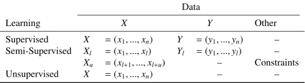
At the core of machine learning lies the analysis of data. Data are worthless unless they contain meaningful information and thus useful knowledge about a particular problem or a set of problems. For different areas of machine learning we can categorise data based on what we know about them, before they are subject to a particular algorithm. The three core types of learning, supervised, semi-supervised and unsupervised learning, differ first and foremost in the type of data they have at their disposal. We highlight these differences in Table 1.
In thesupervisedsetting a set ofnexamplesX=(x1, ...,xn) is provided, along with a set of labelsY =(y1, ...,yn),
resulting in a set of pairs of observationsS = (x1,y1), ...,(xi,yi). In thesemi-supervised setting, the same type of
information is available, however commonly with only a small subset of examplesXl⊂Xwith corresponding labels
Yl ⊂ Y. In contrast to the supervised setting, the amount of unlabelled examplesXu ⊂ X can be fairly large. In
addition, or sometimes instead of the subsetXlof labelled examples, a set of constraints can exist that can be imposed
upon the employed algorithm. Such constraints traditionally denote whether a pair or a set of points should or should not co-exist in the same cluster. Inunsupervised learning the amount of knowledge about data to be analysed is the most restrictive. Only a set ofnexamples fromXis supplied. This makes unsupervised learning hard to define formally and thus a difficult computational problem [41].
One aspect that all three types of learning share is the fact that all sample points should be selected independently and identically distributed from some common distribution on either X, in the case of unsupervised learning, or X×Y in the case of supervised and semi-supervised learning. The restriction on the distribution from which the
∗
Corresponding Author
Table 1: Differences in input knowledge across the three types of learning.
Data
Learning X Y Other
Supervised X =(x1, ...,xn) Y =(y1, ...,yn) –
Semi-Supervised Xl =(x1, ...,xl) Yl =(y1, ...,yl) –
Xu =(xl+1, ...,xl+u) – Constraints
Unsupervised X =(x1, ...,xn) – –
input samples are collected has increasingly been relaxed within the literature and its consequences explored [6]. Importance of incorporation of additional information within machine learning algorithms became more apparent with the introduction of multiple view learning [1, 8] and learning using privileged information (LUPI) [37]. Traditionally such fusion of knowledge was the domain of semi-supervised learning, where techniques such as co-training [3] were employed in order to fuse separate data in order to exploit knowledge encoded within unlabelled data. More recently the inclusion of knowledge from separate hypothetical spaces has also been proposed by Vapnik [36, 38, 37] as part of the supervised setting. In his work the notion of“privileged” and“hidden” information denotes the existence of an additional set of data that provides a higher level information, akin to information provided by a“master”to a pupil, about a specific problem. In the supervised setting such information is only available during training. The fusion of separate hypothetical spaces for the purpose of unsupervised learning, particularly cluster analysis has been investigated in the past [2, 13, 10], however not within the LUPI framework.
In this work we are interested in exploring the idea proposed by Vapnik, however within theunsupervisedsetting. We are particularly interested in the notion of ‘master-class’ learning and the associated learning using ‘privileged’ information which is explained in Section 2. Section 3 provides insights into the difference between information as meant in the traditional sense and the so-called ‘privileged’ information. In Section 4 the question of whether such information can be used to improve data clustering is investigated and a method for combining ‘privileged’ information as part of a clustering solution is proposed. Section 5 highlights the use of our method on a real world dataset. The paper concludes with Section 6 where our results are summarised and future work is proposed.
2. Learning Using Privileged Information
To understand the notion of learning using privileged information, first the wider context of ‘learning from em-pirical data’ is depicted. In machine learning, supervised learning is a subset of learning techniques that have one common goal. This goal is to learn a mapping from inputxto an outputy. The standard input for supervised tech-niques consists of a setX =(x1, ...,xn) ofnexamples from some spaceχof interest. Typically this set of examples
is drawn independently and identically distributed (i.i.d.) from some fixed but unknown distribution with the help of a generator (Gen). Along with such examples we are also given a setY =(y1, ...,yn) of labelsyithat correspond to
our examplesxi. This set is said to have been created by a supervisor (Sup), who knows the true mapping fromx
toy. Thus we are provided with a set of pairs (x1,y1), ...,(xi,yi) and from these we aim to learn the real mapping as
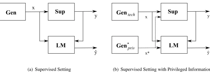
accurately as possible using our learning machine (LM). The general model of learning from examples, adopted from Vapnik [39], can be seen in Figure 1(a). In this figure a generator samples dataxi.i.d. from the unknown distribution of a given problem, which is subsequently paired with an appropriate labelyby the supervisor. The pair (x,y) is then used by the learning machine to learn the mapping fromxtoyin order for the machine to be able to give as similar an answer, to the supervisor, as possible.
Figure 1(b) displays the concept of learning using ‘privileged information’, pertinent to our investigation. In comparison to the supervised setting, there exists an additional data generatorGen∗
privof input datax
∗. This generator
is different from the only generator that exists in the traditional supervised setting and which in this figure is called Gentech. Existence of two separate generators suggests that the inputs xandx∗do not need to come from the same
[image:2.595.141.455.131.217.2]Gen Sup
LM x
y
ŷ
(a) Supervised Setting
Sup
LM
x y
ŷ
Gen Gentech
priv
*
x*
[image:3.595.122.471.125.245.2](b) Supervised Setting with Privileged Information
Figure 1: Two models of learning from examples. In the LUPI setting (b) an additional generator of datax∗exists. This data is called privileged as
it is available only during training.
Originally, Vapnik [36] suggested a learning paradigm called‘master-class’learning, where a teacher plays an important role. This teacher is not the supervisor (Sup) as used in a supervised setting. The teacher is the additional data generatorGen∗priv. In this paradigm the teacher is an entity that provides information akin to information provided by a human teacher. The teacher provides students withhidden information, (x∗). This information is not apparent at first or explicitly stated. It is usually hidden within the actions of the teacher [38]. It provides the students with the teacher’s view of the world. It is available to the students in addition to the information that exists in textbooks and as a result they can learn better and faster. It is important to note that the notion of ‘hidden information’ is different from information hiding in the the field of data hiding [9, 34]. Both areas deal with information passed across a (possibly) covert channel, the purpose and use of such information is however different in both cases.
In [37], Vapnik renamed his learning paradigm to‘Learning Using Privileged Information’. In this formulation the notion of privileged rather than hidden information is presented, where the data is said to be privileged as it is available to us only during training and not during testing.
To realize this advanced type of learning, Vapnik developed the SVM+algorithm [38], where the fusion of priv-ileged information with the classical, technical, data is performed. To understand how this fusion works we refer to the SVM decision function, shown below:
f(x)=(w·z)+b=
n X
i=1
αiyiK(xi,x)+b (1)
In the SVM+method this decision function depends on the kernelK defined in the transformed feature space, however coefficientsαdepend on both the transformed feature space as well as on a newly defined correction space φ(x∗). The correction space is where the privileged data is optimised and thus incorporated as part of the overall solution. Thus in addition to the above decision function, an additional correcting function was introduced [38]:
φ(x∗j)=(w∗·z∗i)+d= 1 γ
n X
i=1
(αi+βi−C)Ki∗,j+d (2)
An important strength of the SVM+algorithm is the ability of the system to reject privileged information in situations when similarity measures in the correcting space are not appropriate, thus privileged information is only used when it is deemed beneficial. One drawback of the system is the increase in computational requirements due to the necessity of tuning of more parameters than in the original SVM setting [37].
More recently Pechyony has analysed the LUPI paradigm theoretically [25, 26]. The LUPI paradigm has also been compared to the problem of structured or multi-task learning in both the classification [20] as well as the regression settings [5]. The multi-task learning framework considers problems where training data can naturally be separated into several groups, which can in turn be used to perform a number of individual model selections. In [20], the authors suggest that the LUPI setting is a similar problem, where training data are structured, however used to create only a single model.
2.1. What is Privileged Information?
To understand the problem that is to be solved in this work, first a description of Vapnik’s“privileged information” needs to be given. Here we will compare it to data as considered in the traditional sense. Vapnik named this traditional data“technical data”, as in most cases such data originated from a technical process, such as a pixel space in the case of a digit recognition task or amino-acid space in the case of classification of proteins. To help us understand what “privileged information” is, it is useful to present examples where such information can become useful. Vapnik suggested three example types of privileged information [37]:
Advanced Technical Model:. In this scenario the privileged information can be seen as a high level technical model of a particular problem to be solved. An example of such a model is the 3D-structure information of proteins and their position within a protein hierarchy in the field of bioinformatics. This 3D-structure is a technical model developed by scientists to categorise and classify known proteins. Technical data on the other hand refers to amino-acid sequences on which classification is performed using most traditional approaches. When information contained within the known 3D-structures can be used to improve learning performed on the amino-acid sequences, without the 3D-structures being required for future predictions, privileged information becomes useful.
Future Events:. Many computational problems involve the prediction of a future event, given a set of current mea-surements. An example of privileged information in this scenario is a set of information provided by an expert in addition to the set of current measurements. For instance if the task at hand is the prediction of a particular treatment of a patient in a year’s time, given his/her current symptoms, a doctor can provide information about the development of symptoms in three, six and nine months time.
Holistic Description:. The last example type of privileged information relates to holistic descriptions [29] of specific problems or problem instances by entities that are associated to the problem domain. Considering a medical problem again where, in this case, biopsy images are to be classified between cancerous and non-cancerous samples, technical data are the individual pixels of each image. Privileged information on the other hand are reports written about the images by pathologists in a high-level holistic language. The aim of the computational task becomes the creation of a classification rule in the pixel space with the help of the holistic reports produced by pathologists, so as to allow for future classifications of biopsy images without the need of a pathologist.
The above three example types of privileged information are only a very small selection of the possible set of additional information that could be obtained from a number of problem domains. Vapnik states that almost any machine learning problem contains some form of privileged information, which is currently not exploited in the learning process [37]. This includes the unsupervised learning process that we are interested in tackling.
3. The Difference Between Information and Privileged Information
Gen
CM
x*
C
Gentech
priv
*
[image:5.595.213.367.129.215.2]x
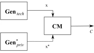
Figure 2: Unsupervised Learning Machine using Privileged Information. In this setting the clustering machine (CM) allows for the fusion of information from both data sources for the purpose of improved clustering.
3.1. Privileged Information in Supervised Learning
In the supervised setting, Vapnik [36, 38, 37] has shown that a learning machine trained with the help of both privileged information, as well as the original technical data, provides improved performance over a machine trained only on technical data. He has also shown that if privileged information is available, the technical data does not need to be of as high quality as when only technical data is used for training. To put this into context, Vapnik compared the classification performance of a learning machine (SVM+) trained on low resolution images of digits with privileged information against a learning machine trained on high-resolution images of the same digits. This comparison has shown comparable results. It is however not known whether privileged information would provide similar type of performance increase when used directly as additional features. Below we demonstrate that there is a difference in combining data from different spaces in ways other than simply concatenating privileged information as additional features to the technical data.
3.2. Privileged Information in Unsupervised Learning
The use of any type of privileged information as part of the unsupervised setting has not yet been performed. In order to show the importance of privileged information, we will highlight its usefulness in the domain of cluster analysis. Figure 2 shows, with the help of the learning machine framework, the unsupervised learning setting using privileged information.
Similarly to Figure 1(b), we have two generators, whereGentechis the generator of the original technical data and
Gen∗privsupplies the learning machine, in this case the Clustering MachineC M, with privileged information. Unlike in the supervised setting there is no supervisor, S up, thus the clustering machine needs to be able to exploit the information encoded within the two data sources, without the knowledge of the number of classes or which instances belong to which group. The clustering machine produces a clusteringC, which provides a set of meaningful partitions ofXaccording to information encoded inxandx∗.
3.3. Clustering Using Perfect Privileged Information
0.0 0.2 0.4 0.6 0.8 1.0 1.2
0.0
0.2
0.4
0.6
0.8
1.0
x
y
● ● ● ● ● ● ● ● ● ● ● ● ● ● ● ● ● ● ● ● ● ● ● ● ● ● ● ● ● ●
● ● ● ● ● ● ● ● ● ● ● ● ● ● ● ●
[image:6.595.210.375.135.285.2]● Class 1 Class 2
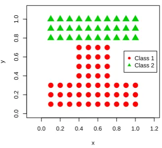
Figure 3: Artificial dataset with true class assignment shown. The dataset is symmetric in point distribution however asymmetric in class assign-ment. This problem cannot be solved using standard clustering techniques.
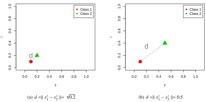
In our case we first assume aperfect expert that can supply information akin to class labels in terms of class separability. By this we mean that the additional information allows for clear separation of the dataset into the correct true clusters. However as this is an unsupervised setting, this additional information cannot be used in the same sense as labels in a supervised setting. Unlike labels, this information cannot be used with a correcting function as there are no guarantees about the correctness of the privileged information and no information about which cluster belongs to a particular class. The information chosen by us for this purpose can be seen in Figures 5(a) and 5(b). Two sets of privileged information were chosen. This information, which we termedpoint-wise, as all points belonging to a class are located at the same location, can be thought of as two dimensional set of points, where each point is associated with an existing data instance of a particular class in the technical dataset. The two sets of data only differ in the Euclidean distance,d, also denoted by the Euclidean normk.k, between points that are representative of the two classes. For simplicity and clarity, privileged information for data items in dataset where the distance between the two classes is d=kx∗
1−x
∗
2k=
√
0.2, that belong to classone(l), areallat location (0.1,0.1), whereas for classtwo(s), privileged information is a set of pointsalllocated at (0.2,0.2). In the second privileged dataset whered =k x∗
1−x
∗
2 k= 0.5,
points belonging to classone(l) areallat location (0.1,0.1) and to classtwo(s) at (0.5,0.4). These two different types of data were chosen to reflect on the fact that the larger the difference between values in different classes, the more separated the two groups become in that particular dimension. Thus if our additional information is very well separated due todbeing very large, then in some cases the problem of separating the two groups becomes easier when concatenating this data in the original feature space. However ifdis small, with respect to other values present in the technical dataset, then even if such attribute is vital for the successful clustering, its influence on the solution will be minimal, especially when the number of dimensions of the technical data set is large with respect to the number of dimensions of the additional data.
3.3.1. Adjusted Rand Index
A clustering validity measure is required to evaluate the performance of the clustering solution provided by all tested clustering algorithms. A method called the adjusted Rand index [17] was employed to assess the similar-ity between the clustering solutions produced by the clustering algorithms and the true solution. This method is a corrected-for-chance version of the RAND index [28], which assesses the degree of agreement between two partitions of the same set of data. The method has a maximum value of 1, which denotes a perfect agreement between the two tested partitions. The minimum of 0 denotes that the two sets do not agree on any pairs of points.
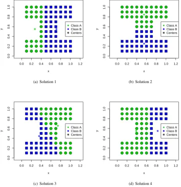
3.3.2. Clustering of X Concatenated with X∗- (X+X∗)
0.0 0.2 0.4 0.6 0.8 1.0 1.2
0.0
0.2
0.4
0.6
0.8
1.0
x
y
● ● ● ● ● ● ● ● ● ● ● ● ● ● ● ● ● ● ● ● ● ● ● ● ● ● ● ●
● Class A Class B Centers
(a) Solution 1
0.0 0.2 0.4 0.6 0.8 1.0 1.2
0.0
0.2
0.4
0.6
0.8
1.0
x
y ● ● ● ●
● ● ● ● ● ● ● ● ● ● ● ● ● ● ● ● ● ● ● ● ● ● ● ● ● ● ● ● ● ● ● ● ● ●
● Class A Class B Centers
(b) Solution 2
0.0 0.2 0.4 0.6 0.8 1.0 1.2
0.0
0.2
0.4
0.6
0.8
1.0
x
y
● ● ● ● ● ● ● ● ● ● ● ● ● ● ● ● ● ● ● ● ● ● ● ● ● ● ● ● ● ● ● ● ● ● ● ● ● ●
● Class A Class B Centers
(c) Solution 3
0.0 0.2 0.4 0.6 0.8 1.0 1.2
0.0
0.2
0.4
0.6
0.8
1.0
x
y
● ● ● ● ● ● ● ● ● ● ● ● ● ● ● ● ● ● ● ● ● ● ● ● ● ● ● ● ● ● ● ● ● ● ● ● ● ● ● ● ● ● ● ● ● ● ● ●
● Class A Class B Centers
[image:7.595.116.471.233.599.2](d) Solution 4
0.0 0.2 0.4 0.6 0.8 1.0 0.0 0.2 0.4 0.6 0.8 1.0 z i ● ● ● ● ● ● ● ● ● ● ● ● ● ● ● ● ● ● ● ● ● ● ● ● ● ● ● ● ● ● ● ● ● ● ● ● ● ● ● ● ● ● ● ● ● ●
● Class 1 Class 2
d
(a) d=kx∗1−x∗2k=√0.2
0.0 0.2 0.4 0.6 0.8 1.0
0.0 0.2 0.4 0.6 0.8 1.0 z i ● ● ● ● ● ● ● ● ● ● ● ● ● ● ● ● ● ● ● ● ● ● ● ● ● ● ● ● ● ● ● ● ● ● ● ● ● ● ● ● ● ● ● ● ● ●
● Class 1 Class 2
d
[image:8.595.116.469.134.309.2](b)d=kx1∗−x∗2k=0.5
Figure 5: Point-wise privileged information,x∗, supplied in addition to original technical data,x. Hereddenotes the Euclidean distance between
the points in the two classesx1andx2. Each class contains as many items inx∗as there are items inx, however as these are all located at the same
position in this scenario, only one item per class can be seen in this figure.
index method is calculated across 100 runs of the algorithm. As stated earlier the results of the first experiment confirm that the algorithm cannot find the correct solution and that in many cases it finds a completely wrong solution. Concordance of 62% between the K-Means solution and the true class assignment is found in the best case, with a mean concordance of 52%. On the other hand the worst solution finds no agreement between the true clustering and the solution that K-Means found. This is due to the fact that the algorithm is susceptible to local optima, which are typically found when the initial centres of the algorithm are not chosen optimally. As the K-Means algorithm traditionally selects such initial centres at random, it is understandable that many of the algorithm’s solutions might be incorrect. Numerous solutions to this initialisation problem of the K-Means algorithm have been proposed in the past, for example [4, 23, 21], however we are not interested in solving this problem per se, nevertheless our analysis does have implications that are related.
Once the results obtained on the original technical data,X, show that the K-Means algorithm cannot achieve a very good solution, we now include the privileged information as a part or in addition to the original feature space.
In the first instance we obtain results for the clustering produced by K-Means when the privileged information is fused into the feature space of the technical data. Hence the additional data is simplyappendedto the original dataset, and thus can be thought of as only an additional set of attributes. We will refer to this scenario throughout the rest of this paper using the following notation:X+X∗, where+denotes a concatenation of the two sets of data, resulting in one dataset. To evaluate whether significant differences exist in the results, we examine our results with the help of a statistical test called the Wilcoxon signed-rank test [42]. A confidence interval level of 0.05 was chosen and a null hypothesis with two alternative hypotheses was given.
By including the additional information as simply another set of attributes we observe that across 100 runs the quality of solutions of the K-Means algorithm in the case whend =
√
0.2 slightly decreases, from 0.52 to 0.51, when looking at the mean adjusted Rand index value. Comparing the clustering of X with clustering of X+X∗ statistically, we cannot reject any of our proposed three hypotheses. The null hypothesis states that the two results are the same. The two alternative hypotheses state that the distribution of either one or the other result has a shift to the right with respect to the distribution of the other result. The statistical analysis suggests that the two results are not statistically significantly different. Thus there is no evidence for the benefit of using the additional information from X∗by combining it withXfor the case whend= √0.2.
additional information helps to sufficiently separate the two groups, making correct solutions possible. In this case we cannot, however, call this additional information privileged because it is simply an additional set of features. Here the fusion ofX+X∗provides enough separation that influences the K-Means algorithm by a sufficient amount. The two attributes from the technical space now comprise only 50% of the information based on which the K-Means algorithm makes a decision. The other 50% comprises of the additional information which can be thought of as perfect with a high level of separability due tod=0.5. This result highlights the importance of separability of classes based on the separability of individual features within an analysed dataset. As our original dataset comprises of two dimensions and the privileged dataset is also two dimensional, if the privileged dataset on its own is well separated, this has great influence on the analysis of the combined dataset, especially in cases where the dimensionality ofX does not differ greatly from the dimensionality ofX∗. In cases where the dimensionality of the technical data is substantially larger than the dimensionality ofX∗, then even ifX∗is perfectly linearly separable, the data inXwill degrade the influence of the information inX∗.
It is also important to note that if our data is always as clearly separable as in this example, then we can always obtain very good solutions using traditional methods. The above optimal case is however rarely to be experienced. Furthermore, distinct separation is difficult to obtain if our privileged information includes substantial noise, similar to that of the technical data. A question begs whether the fact that our privileged information comes from the same domain, rather than the same distribution, can be of benefit. In answering this question and help us overcome the above mentioned issue of dimension dependent separability, we used privileged information in a way that fuses knowledge from the two separate data sources, however not in the feature space of the technical data.
3.3.3. Clustering Consensus of Disparate Hypothetical Spaces - aRi-MAX
As both technical data and privileged data essentially come from the same domain, they should provide an insight into the problem that we are trying to analyse. In terms of clustering, the two datasets should provide information about the same or similar sets of clusters that belong to the given domain. Assuming the above is true, when each dataset is clustered individually, we should be able to achieve a consensus of the two results. Consequently we should understand better the underlying structure of the analysed data. The field of consensus clustering, sometimes also called aggregation of clustering [33, 35, 14], addresses a similar problem, where a number of clusterings of the same dataset exists and a consensus between those is sought after. Here we are interested in the clustering of two datasets that come from the same domain but different generators. In this section we use the clustering of the privileged information to select the best possible clustering of the technical data. We have devised an algorithm, called aRi-MAX, for this purpose. Pseudo-code foraRi-MAXis shown in Algorithm 1.
Algorithm 1:aRi-MAX - Clustering consensus ofXandX∗using adjusted Rand index. Input: Technical DataX, Privileged DataX∗
Output: Clustering ofX, maximizing agreement betweenXandX∗ 1 initialization;
2 foreachi in Runsdo 3 Cti←clust(X); 4 Cei←clust(X∗);
5 end
6 foreachi in Ctido
7 Cci←max(adjustedRandIndex(Cti,Ce))
8 end
9 max(Cci)
0.0 0.2 0.4 0.6 0.8 1.0 0.0 0.2 0.4 0.6 0.8 1.0 z i ● ● ● ● ● ● ●● ● ● ●●● ● ● ●● ● ● ● ●● ● ● ● ● ● ● ● ●●● ● ● ● ● ● ● ● ●● ● ● ● ● ●
● Class 1 Class 2
(a)d=kµ1−µ2k=
√
0.2,σ=0.6
0.0 0.2 0.4 0.6 0.8 1.0
0.0 0.2 0.4 0.6 0.8 1.0 z i ● ● ● ● ● ● ● ● ● ● ● ● ● ● ● ● ● ● ● ● ● ● ● ● ● ● ● ● ● ●● ● ● ● ● ● ● ● ● ● ● ● ● ● ● ●
● Class 1 Class 2
[image:10.595.116.468.134.307.2](b)d=kµ1−µ2k=5,σ=1.5
Figure 6: More realistic, Gaussian noise based privileged information,X∗. This privileged information is more akin to data in real-world scenarios,
where numerous data items from different classes overlap, making a separation of the classes more difficult.dagain denotes the Euclidean distance between the centres of the two existing classes andσdenotes the standard deviation.
highest agreement are selected as the final solution candidate, steps6-9in 1. Once this is completed, the candidate clustering solution of the technical dataset is evaluated against the true solution.
3.3.4. Clustering by Fusion of X with X∗- (XX∗)
The fusion ofXandX∗by means of ouraRI-MAXmethod as well as our future fusion methods shall be denoted in the following way,XX∗. Here however the termshall not be interpreted in the strict mathematical sense denoting
congruence. The choice of this symbol was due to the fact thatXandX∗essentially should provide a congruent view of the same problem domain.
Experiments using theaRI-MAX method were performed on X X∗, for both the d =
√
0.2 and thed = 0.5 cases. Results obtained show that across the one hundred runs we are now able to obtain the best achievable result, given the dataset and clustering algorithm, 100% of the time in both cases. Thus the average agreement between the correct clustering and our solution across the 100 runs is 0.62. Even though the performance of ouraRi-MAX method is limited by the capability of the underlying clustering technique applied on the technical data,X, in the case of K-Means, the variability of the outcome of the algorithm is reduced from a standard deviation (σ) of 0.23 for the d=
√
0.2 case and 0.1 for thed=0.5 case toσ=0 in both cases when ouraRI-MAXmethod is used. Statistical tests performed reveal that obtained results are statistically significant and that the distribution of the results of our method were shifted to the right from the distribution of the results obtained on both the original data,X, as well as on the combined data,X+X∗, fused in feature space in thed =
√
0.2 case. These results confirm that the use of privileged information, in a way different than as part of the original feature space, is a viable direction.
3.4. Clustering Using Imperfect Privileged Information
Table 2: Results of statistical analysis of performance of K-Means algorithm on technical data,X, versus fusionX+X∗and theaRi-MAXmethod on XX∗.Gaussianprivileged information withd=kµ
1−µ2k=
√
0.2. Statistical test performed is Wilcoxon signed-rank test at the 0.05 confidence interval level.
Clustering R1=R2 R1<R2 R1>R2
R1 R2 p-value reject? p-value reject? p-value reject?
X vs. X+X∗ 0.08318 no 0.04159 yes 0.9599 no
X vs. XX∗ 0.00024 yes 0.9999 no 0.00012 yes
X+X∗ vs. X
X∗ 4.207e-05 yes 1 no 2.104e-05 yes
3.4.1. Clustering of X Concatenated with X∗- (X+X∗)
When this more noisy type of additional knowledge is fused with the technical data in the original feature space, X+X∗, in thed =
√
0.2 case, the results of the K-Means clustering algorithm slightly degrade to 48% compared to using only technical data,X, where a result of 52% is achieved. Again in the case whered =0.5, the overall perfor-mance improves, however this time not as dramatically as in the point-wise dataset case with an average concordance of 91% rather than 97%. Statistical tests were also performed on the results obtained from the new fusions of data using Gaussian privileged information. From these tests it is apparent that ford= √0.2 we reject the hypothesis that the distribution of the result of the fusedX+X∗space is shifted to the right of the result on X. Therefore we can conclude that in this example the addition of privileged information by means ofX+X∗provides an inferior solution.
3.4.2. Clustering by Fusion of X with X∗- (X
X∗)
By using our aRi-MAX method, results show a dramatic improvement with regards to the consistency of the solutions. Even if the information in the privileged dataset is obscured by noise, a more consistent solution using the K-Means algorithm was achieved withσ = 0 for both cases of privileged information. To evaluate the results statistically we performed the Wilcoxon paired signed-rank test again and summarised the results in Table 2 for the d= √0.2 case.
These results show that addition of privileged information to the technical data byX+X∗has negative effect on the capability of the K-Means algorithm. Conversely, the use of the proposedaRi-MAXmethod gives results that surpass other results in consistency and therefore in performance. For the case whend =0.5, the statistical results confirm that the fused privileged data in the original technical space provides the K-Means algorithm enough information for achieving a very good solution in the majority of performed runs.
4. Can Privileged Information Improve Clustering?
H(X)
H(Y)
I(X;Y)
H(X|Y)
H(Y|X)
[image:12.595.185.412.115.266.2]H(X;Y)
Figure 7: Depiction of the relationship between various information theoretic concepts. H(X) and H(Y) denote entropy of variables X and Y respectively. H(X|Y) denotes the conditional entropy of X given Y. H(X;Y) is the joint entropy of variables X and Y and I(X;Y) is the mutual information of the aforementioned variables.
4.1. Information Theoretic Approach
Information theory deals with the quantification of information. It was originally inspired by a subfield of physics called thermodynamics, where the measure of uncertainty about a system is measured using a concept calledentropy. Entropy in this case is the amount of information that is necessary for the description of the state of the system. At a lower level, entropy is the inclination of molecules to disperse randomly due to thermal motion. The more disper-sion, the larger the entropy [15, 12]. Ludwig Boltzman devised a probabilistic interpretation of such thermodynamic entropy,
S =klogW (3)
where the entropy of the systemS is the logarithmic probability of its occurrence, up to some scalar factor, k, the Boltzmann constant. Subsequently it was observed that the properties of entropy can be found across many different fields of science. Claude E. Shannon introduced in 1948 the concept of entropy for the purpose of communication over a noisy channel [31], which started the field of information theory. In our work we are dealing with Shannon’s concept of entropy and its subsequent variations and derivations.
From the information theoretic point of view entropy is defined as follows,
H(X)=−
n X
i=1
p(xi) logbp(xi) (4)
whereH(X) is the entropy of a random variableX andp(x) is the probability mass function of an instance xof X. Georgii [15] states that entropy should not be considered a subjective quantity. Entropy is essentially a measure of the complexity inherent inX, which describes an observer’s uncertainty about the variableX. Now considering we have two random variables and we would like to find out the information that the two variables share. In other words we would like to know the mutual dependence of variableX on variableY. For this purpose the following calculation, calledMutual Informationexists,
I(X;Y)=X
y∈Y X
x∈X
p(x,y) logb p(x,y) p1(x)p2(y)
(5)
modi-fied version of the Mutual Information concept, now normalised to return values in the range [0,1], has been proposed,
N MI(X,Y)= √I(X;Y)
H(X)H(Y) (6)
In this equationI(X;Y) denotes the Mutual Information between variablesXandY.H(X) andH(Y) denote the entropy of variablesXandY respectively.
The above information theoretic method provides a way to measure and compare the levels of information across different variables. This provides a tool that allows for an insight into combining separate sets of data and extracting the necessary segments of such data that could contribute to an improved solution, without the need for explicit class labels.
4.2. Dot Product Ratio Measure
To account for information encoded in the privileged dataset, a method has to be devised that is able to discern which group or cluster should be affected by the information inX∗. As our data does not have labels, such processing can only take place according to similarity or consensus between solutions of two or more methods that provide us with their understanding of the underlying data structure. In section 3.3, we have proposed a method to evaluate a number of solutions of the K-Means algorithm, run on the two disparate datasets. In this case one dataset, the technical data, is considered as the dominant set. The solution found for the privileged dataset is only used to find an agreement in order to select the most similar solution for thedominantset. An apparent issue arises with this method however. In cases where both solutions end in local minima, this might result in an agreement between the two solutions that is stronger than a more accurate solution, which does not agree strongly across the two datasets. The use of methods which do not have issues with local minima partially resolves this issue. Also ouraRi-MAXsolution only selects the best solution from the technical dataset. It does not provide for an improvement, based on the privileged information. Thus if data inX∗ holds information that is not encoded inX, we cannot exploit this. For this reason we must go beyond consensus and attempt to use data inX∗to amend the solution ofX.
The first problem with attempting this is how a solution can be affected in a general enough manner to make our method applicable across a wide variety of clustering methods. If we adapt the approach taken by Vapnik [37], we are posed with a number of difficulties. First of all, as mentioned above, we do not have labels. Secondly in order to affect a decision boundary in a similar manner to SVM+, we need to be able to empirically assess our level of correctness of assigning a data item to a specific cluster. Without labels this is impossible. However even if this was possible, for some algorithms this does not pose a reasonable solution. When considering our artificial dataset, the amendment of the cluster centres found by the K-Means algorithm shifts the decision boundary toward a solution which in this case might be correct, however this only works when our data is linearly separable. Any movement of the cluster centres affects the decision boundary, which when moved, might lower the quality of the final solution overall. Thus rather than directly affecting a decision boundary or a cluster centre, we propose to generate additional dimensions or attributes, which encode the best possible solution of a clustering algorithm on the privileged data. In this manner we can try to avoid the issue of linear separability as a non-linear problem might become linearly separable in some arbitrary high dimensional space [30].
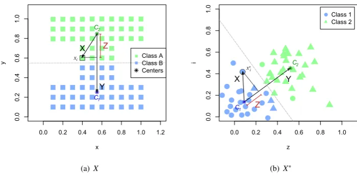
The issue of which cluster should be affected by information inX∗is still pertinent however. In order to deal with this we propose to use adot-productbased ratio measure which evaluates whether an item inXis more likely to have been correctly clustered than a related item inX∗. Our approach is depicted in Figure 8, which shows how a feature vectorxiis being evaluated against the clustering onXandX∗and the relative ratio of the location of this vector with
respect to its assigned cluster centres is used to determine whether the data item is classified correctly or whether its class should be changed and re-evaluated.
More mathematically we are concerned with calculating the distance of the point xi projected onto a plane
con-necting the two cluster centresC1andC2. To perform such operation we use the dot product,
X·Y =|X||Y |cosθ (7)
whereXdenotes a vector in the mathematical sense, originating atC2and connectingxi.Yis a vector connecting
0.0 0.2 0.4 0.6 0.8 1.0 1.2
0.
0
0.
2
0.
4
0.
6
0.
8
1.
0
x
y
Z
Y X
C1
C2
xi Class A
Class B Centers
(a)X
0.0 0.2 0.4 0.6 0.8 1.0
0.
0
0.
2
0.
4
0.
6
0.
8
1.
0
z
i
Class 1 Class 2
C1
C2
X Y
Z
x*i
[image:14.595.116.466.136.308.2](b)X∗
Figure 8: Depiction of the dot product ratio measure used to determine whether an assignment of an input feature vector is more likely to belong to a cluster as determined by clustering ofX(a) or to a cluster as determined by clustering ofX∗(b). In our approach this decision depends on the
comparison of relative ratios of distance from the vector’s assigned cluster centre for each clustering. In this figureYdenotes a vector connecting the two cluster centres,Xdenotes a vector connecting inputxiwith the closest cluster centre andZdenotes the projection ofXontoY.
value of this angle, we use the dot product form which calculates the projectionZusing the known lengths ofXand Yas follows,
Z= X·Y
Y·YY (8)
To calculate the necessary ratio which allows us to evaluate how correct a clustering solution might be for a particular pointx, we perform the following calculation,
Rd(x)=
kZ−Ckk
kZ−Ck+1k
(9)
whereRd(x) denotes the function that calculates the distance ratio onx,Z denotes the projection of the currently
examined inputxionto the vectorXandCkandCk+1are the assigned cluster centre and the closest subsequent cluster
centre respectively. In cases where we only have two clusters,Ck+1denotes the cluster centre to whichxihas not been
assigned, in other words the opposing cluster centre. In cases wherek>2 the cluster centreCk+1is the closest cluster
centre according to some metric, such as the Euclidean distance or the topographic distance in the SOM algorithm. In our experiments we only deal withk=2 to simplify our analysis. The symbolk.kdenotes the Euclidean norm and in our calculation the distance between the projected locationZ from its assigned cluster centre as well as from the opposing cluster centre. The projection of pointxiis calculated according to Equation 8 as follows,
Z = (xi−Ck)·(Ck+1−Ck) (Ck+1−Ck)·(Ck+1−Ck)
(Ck+1−Ck) (10)
wherexidenotes our input vector of interest andCkandCk+1again the cluster centres computed by a clustering
al-gorithm. To put this calculation into perspective the pseudo-code for our method, calledP-Dot, is shown in Algorithm 2 and explained in detail in the next paragraph.
4.3. Privileged Information Dot Product Consensus:P-Dot
Algorithm 2:P-Dot Algorithm Input: Technical Data:X Input: Privileged Data:X∗ Output: Clustering ofX 1 initialization;
2 foreachiiniterdo /* Consensus Step */
3 Ctechi←clust(X);
4 Cprivi←clust(X∗);
5 end
6 foreachiinCtechido
7 Cbestp←max(NMI(Ctechi;Cprivi)) ; /* Mutual Information */
8 end
9 Ctechbest←which(max(Cbestp));
10 Cprivbest←max(Cbestp);
11 ifNMI(Ctechbest;Cprivbest)<min(H(Ctechbest);H(Cprivbest))then
12 ifdifferences>matchesthen /* Fusion Step */
13 xi←matches(Ctechbest;Cprivbest);
14 else
15 xi←differences(Ctechbest;Cprivbest);
16 end
17 foreachiinxido
18 ifRd(Ctechbest[xi])>Rd(Cprivbest[xi])then /* Ratio Measure */
19 swap.cluster.assignment(Ctechbest[xi]);
20 end
21 end
22 Xnew←bind(X,Ctechbest[A],Ctechbest[B]);
23 Cf inal←clust(Xnew);
In Algorithm 2 lines 2 to 10 highlight an amended version of our consensus method described in section 3.3. Instead of using the Adjusted Rand Index method, we employ here the Normalised Mutual Information (Equation 6) to find two most similar clusterings amongst a set of solutions. Strehl and Ghosh [33] have shown that this measure is a suitable way of comparing clusterings with some advantages over the Adjusted Rand Index method, such as the absence of strong assumptions on the underlying distribution. Steps 11 to 24 outline each step of theP-Dotmethod. Initially the results of the best clustering solutions are evaluated for similarities at steps 12-16. If the two clusterings are identical, then no improvement can be obtained. If there exist differences between the solutions, we determine whether there are more differences than similarities between the two solutions (lines 12-14) or vice versa (lines 15-16). This is due to the fact that explicit cluster labels are meaningless and thus cluster A onX can be called cluster B inX∗. For this reason we only need to deal with the smaller set of values, whether they are matching labels or dissimilar labels. Then for each match or mismatch (line 17), the dot-product ratioRd(x) is calculated (line 18) for
both inputs fromX andX∗, to determine which of the two solutions is more likely to be correct. If the solution on spaceX∗is more likely to be correct, the label of the corresponding item in the solution ofXis inverted (fork=2), at step 19. Once this procedure is completed,knew attributes are created, one per each cluster found (line 22). These attributes are filled with maximum normalised values for data items that belong to that particular cluster according to the labels as decided in the previous step. Eventually a new datasetXnewis generated. This data is clustered again and
its solution is the final solution of our method (line 23). What this approach achieves is in effect taking into account data streams separately and treating them uniquely. This allows for data that might normally be deemed irrelevant due to swamping, to become equally important in the final processing of the dataset.
4.4. Experimental Evaluation
To evaluate our proposed method empirically we employ our artificial dataset from paragraph 3.4. The K-Means clustering algorithm is used within theP-Dotmethod and compared against our previousaRi-MAXmethod as well as a set of four established clustering methods. These methods are the Expectation Maximization algorithm [11], which is a probabilistic algorithm that fits Gaussian models onto the dataset, Spectral Clustering [32, 22], which transforms the original data into another space within which the actual clustering is performed. Also two versions of the SOM [18] algorithm are employed. One method that treats the SOM as a clustering algorithm assigning one node per cluster, similarly to K-Means and another method which specifies a larger number of nodes that are shared between clusters present within the dataset. These nodes are subsequently clustered using the K-Means algorithm in the same way as was performed by Vesanto and Alhoniemi in [40]. The mixture ofX+X∗, combined in the same feature space is used as the dataset on which the comparison techniques are employed.
First ourP-Dotmethod is tested on the artificial dataset with point-wise (perfect) privileged information. In both cases (d =
√
0.2 andd = 0.5) the performance of our new method is superior to the aRi-MAX method. The P-Dotmethod achieves almost 100% accuracy in both cases, compared to 62% performance of theaRi-MAX method. Subsequently when the more complex Gaussian based privileged information is tested, again our new method achieves very good results in both situations. An average concordance of 85% and 95% for thed=
√
0.2 andd=0.5 cases are achieved, respectively. This is an improvement of 23% and 33%, respectively, over theaRi-MAXmethod.
When compared to other existing techniques, such as the SOM, Spectral Clustering and Expectation Maximization algorithms, we can see that our method is still superior in both cases where privileged information is more complicated (d= √0.2). Box plots for these results can be seen in Figures 9(a) and 9(b) respectively.
Table 3 highlights a summary of statistics for all of the tested algorithms on the Gaussian privileged dataset with d= √0.2. It is apparent that ourP-Dotmethod outperforms all others in all aspects except possibly stability. However the standard deviation of the results for our method is still very low. Best results in this table have been underlined for the purpose of clarity.
5. P-Dot in the real world
Table 3: Statistical information on the performance of theP-Dotmethod compared to various clustering techniques applied toX+X∗using the
Gaussian based privileged information withd= √0.2 (Figure 6a). The values show the normalized mutual information between clusters found using a given method and the true class labels across 100 runs. 1 denotes perfect match and 0 denotes no matches at all. Best results have been underlined.P-Dotperforms best overall. SOM2K denotes the combination of SOM and K-Means according to [40].
Min Max Mean Median St.Dev.
K-Means (X) -0.0129 0.6184 0.4719 0.6184 0.2623
K-Means (X+X∗
) -0.0129 0.6184 0.5373 0.6184 0.2109
aRi-MAX 0.6184 0.6184 0.6184 0.6184 0.0000
P-Dot 0.8462 0.8960 0.8472 0.8462 0.0070
EM 0.7979 0.7979 0.7979 0.7979 0.0000
Spectral 0.6184 0.7979 0.6902 0.6184 0.0884
SOM 0.6184 0.6184 0.6184 0.6184 0.0000
SOM2K -0.0162 0.7054 0.4395 0.5770 0.2629
0.0
0.2
0.4
0.6
0.8
1.0
Adjusted
R
AND Inde
x
K-Means SOM SOM2L EM SpecC P-Dot
(a) Point-wise Privileged Information
0.0
0.2
0.4
0.6
0.8
1.0
Adjusted
R
AND Inde
x
K-Means SOM SOM2L EM SpecC P-Dot
(b) Gaussian Privileged Information
[image:17.595.160.433.493.638.2]28x28 pixel Digit Images
(a) 28∗28 pixel digit dataset
10x10 pixel Digit Images
[image:18.595.173.429.112.233.2](b) 10∗10 pixel digit dataset
Figure 10: Subset of the MNIST digit dataset comprising of 100 digits at two different resolutions, providing different levels of information. The lower the resolution, the more information is potentially lost. The dataset comprises of two classes of digits, the numbers 5 and 8 and variations thereof. There are 50 examples of each class.
5.1. The Task of Digit Recognition
The task of digit recognition is one of the most frequent pattern recognition tasks. Numerous research papers and results have been generated on this topic, particularly within the supervised learning community. The MNIST database of handwritten digits [19] is an eminent source of such research1. Vapnik [38] used a subset of the MNIST dataset comprising of 100 digits from two different groups. The two groups are 50 variations of the digit 5 and 50 variations of the digit 8. Each digit is originally a 28*28 pixel gray-scale image, seen in Figure 10(a). Thus an image can be thought of as a 784-dimensional feature vector with values in the range [0−255]. To make the task of classification slightly more difficult, Vapnik created a second dataset, based on scaled down versions of the original images. Thus a set of 100 gray-scale images at a resolution of 10*10 pixels has been created, seen in Figure 10(b). This dataset can again be thought of as a 100-dimensional dataset with a range [0−255].
5.2. Privileged Information
To explore the notion of learning using privileged information, such type of additional information had to be created. In order to do this Vapnik et al. [38] created a set of poetic descriptions with the help of language experts. By poetic description we mean a description of what the expert saw and interpreted using his own words in the form of a poem. An example of such a description follows:
Poetic Description:“Item.4 - A two-part contradictory creature. One part is rounded, the other is a bit angular. The bottom is on the earth (steadier than the first three figures). Open and free for the wind. It is slightly slanted to the right. The upper part is broken. It has a small gap. Insignificant. The lower round part has no “hill”. The man throws a stick. He goes headfirst. He looks ahead - where is the stick? He is attacking somebody or training. The wriggling snake is beating its tail. The unpleasant movement. Not so nice. A bit irregular. Not so clear. A rope. Asymmetrical. No curlings of the ends.”
In addition to this description a separate interpretation of the digits has also been created. Rather than a subjective description of the emotive impact of each digit on the observer using arbitrary words, the second set of privileged information has been created using words of opposing meanings. For this purpose this set of privileged data is termed Ying Yang2. An example of this type of data follows:
Ying Yang:“Item.3 - Very sociable creature between 30 and 40. Everything is normative and right-ful. Masculine firmness in everything. May be dull and uninventive but good-natured. Seeking nothing. It is still water but useful with all the usual advantages. Take your time - you can live nearby and be happy. Nothing mysterious about it. You see the bottom, the water is so transparent. Simplicity may be its strong side.”
1The MNIST dataset can be downloaded from http://yann.lecun.com/exdb/mnist/. This website also contains a summary of the best published
classification results of various supervised algorithms using this data
● ● ● ● ● ● ● ● ● ● ●
● ● ● ● ● ● ● ● ● ● ● ● ● ● ● ●
● ● ● ● ●
● ● ● ● ●
● ● ● ● ●
●
10 * 10 X 28 * 28 X Poetic X* Ying Yang X*
0.0
0.2
0.4
0.6
0.8
1.0
Adjusted RAND Inde
[image:19.595.223.364.127.248.2]x
Figure 11: Analysis of the K-Means algorithm onXitself as well as on both sets of privileged dataX∗on their own. It is apparent that the higher resolution data contains more information, useful for better clustering. The PoeticX∗data is not a useful resource of information on its own when clustered using K-Means. The opposite is true for the Ying YangX∗, which allows for correct identification of the two true clusters on its own.
To make these additional sets of data usable in computation, the text has been analysed and a set of keywords that occur across the dataset have been extracted. An example of such a keyword is “Upright”, which captures whether a digit is slanted or not, or “Gaps”, which measures the amount of gaps a digit has. For each keyword a scale of the term’s possible range of meaning has been proposed. In our example keywords “Upright” has a binary value and “Gaps” has a scale from 0 to 5. Finally a 21-dimensional vector has been created for each digit encoding the poetic description of each digit and a 31-dimensional vector has been created for the Ying Yang dataset3.
5.3. Clustering Performance
To evaluate the capability of our proposedP-Dotmethod, we have used the above described dataset and performed a number of experiments. We have run each algorithm 100 times to ensure better consistency for the comparison of results. First we used the K-Means algorithm and clustered each individual dataset on its own, to understand how well each dataset can segment the data into the correct categories. The result of this clustering, Figure 11, provides an insight into the approximate level of information encoded within the datasets that can be revealed using the K-Means method. The higher resolution version of the data gives a slightly better insight into the data’s underlying structure and thus the K-Means performs better in this scenario, by approximately 3%. When looking at the privileged information, we observe that there is a dramatic difference between the two sets of data. The poetic description of each digit reveals very little on average, with a hint that in cases when the K-Means algorithm starts with a good set of initial values it is possible to achieve clustering that has an agreement of at maximum 38%. On the other hand when looking at the Ying Yang privileged information we can see that the dataset can be categorised into the two required groups with 100% accuracy, consistently, using just the privileged information. From a logical point of view this difference between the privileged information makes sense as the Ying Yang descriptions seek to evaluate visual features that are contradictory and thus aim at describing each digit at extreme ends of the description scale. For our analysis we are mainly interested in exploring the benefit of privileged information with a discrimination ability such as the poetic dataset as we believe such type of additional information, which is insufficient on its own to solve the task, is more likely to occur in many real-world situations.
Subsequently an evaluation of the clustering performance of the K-Means dataset on the fusionX+X∗is required to be able to assess if such a combination provides good enough results on its own. The data has been standardised using the min-max method [27, 16] in order to ensure that no swamping of attributes can occur. The result of the K-Means clustering on the normalised version of the spaceXcan be seen in Figure 12. The fusion of the technical and the privileged data resulted indecreasingthe quality of the K-Means solution in both cases by up to 6%. Thus we can assume that without any further processing the additional information in the original feature space only hinders
3The reader is referred tohttp://www.nec-labs.com/research/machine/ml website/department/software/learning-with-teacher/ where a detailed
● ● ● ●
● ● ● ● ● ● ●
● ● ● ●
● ●
● ● ● ● ● ● ●
● ● ●
● ● ●
●
● ● ● ● ● ●
X X+X* P−Dot X X+X* P−Dot
0.0
0.2
0.4
0.6
0.8
1.0
Adjusted RAND Inde
x
[image:20.595.148.440.127.279.2]10 * 10 pixels 28 * 28 pixels
Figure 12: Comparison of results of the K-Means algorithm and theP-Dotmethod on the digit dataset. Results for individual clusterings ofXfor both versions of the normalised datasets as well as the clustering on the fusedX+X∗data using K-Means are shown. TheX+X∗fusion clearly degrades the performance of the K-Means algorithm. Results of theP-Dotmethod using PoeticX∗on the other hand show an improvement over K-Means in both situations. An improvement overXand more dramatically overX+X∗is apparent.
our search for a good solution. This highlights the necessity of processing such data in a unique way that allows for the extraction of information fromX∗that can improve the final cluster, but notdegradeit.
Knowing that privileged information fused within the feature space of the technical data does not bring any benefit to cluster analysis, ourP-Dotmethod is employed to assess the benefit of data fromX∗combined in our unique way. For the lower resolution dataset we observe that our method provides an improvement over both,Xonly, as well as the fusedX+X∗, seen in Figure 12. This is the case for both the mean performance across the 100 runs, where an improvement of 5% with respect to clustering onXis observed and 11% with respect toX+X∗. The best possible attainable solution also improved in this case. In the case of the higher resolution version, there is an improvement of 1% with respect toXand 6% with respect toX+X∗. This is a promising result as we only want to improve upon a solution in case the privileged data can provide such benefit. When such improvement is unattainable from the additional dataset, we do not want to negatively affect our existing solution. Wilcoxon signed-rank statistical test was performed, confirming these results. Very small p-values for the two-sided tests reject the hypothesis that the two results are the same. Analysis of the alternative hypotheses help us clearly identify that ourP-Dotmethod has better results in both cases.
5.4. The Importance of Dimensionality Reduction inP-Dot
structure. In our next experiment we have employed the PCA technique on the technical data in order to reduce the dimensionality from 784 dimensions to only two. Our experiments have shown that such a transformation does not hinder greatly the clustering capability of the K-Means algorithm with respect to clustering onX. On the contrary the reduction has selected the most relevant features of theX +X∗data which more clearly reveal the underlying structure and thus improve performance with respect to the clustering onX+X∗. When the PCA is used onX as part of ourP-Dotalgorithm, there is no apparent difference for the lower resolution dataset with respect to theP-Dot method on normalisedX. On the other hand the higher resolution dataset benefits significantly from this reduction and theP-Dotmethod can have greater influence on the final clustering result. This results is a further improvement of approximately 5% on top of theP-Dotmethod on normalisedX. Statistical tests were performed on all results to confirm their validity.
We believe that there is a fundamental issue that needs to be addressed that is missing from many machine learning experiments. The fact that ourP-Dotmethod could improve upon the solution of a traditional method on the same dataset, using only a form of an agreement and subsequent encoding of such an agreement within a dataset that is re-evaluated, hints at the possible importance of not only the notion of privileged information, but more interestingly on the importance of different generators of data. Privileged information can be thought of as simply an additional set of attributes that describe a given problem. Our analysis above however showed that when adding such data to existing technical data in the traditional way, no benefit is apparent. What is necessary for this data to become useful is, we believe, the relative importance of the information encoded within, to be treated with equal weight as data from any other source, independent of dimensionality. In other words, one attribute from a separate source or generator of data should be treated equally to any number of attributes from another, but single source.
5.5. Comparison with Other Clustering Techniques
To contrast ourP-Dotmethod with other existing clustering techniques, we have applied the same set of clustering algorithms used in section 4.4 to the digit datasets. An overview of the results obtained for the digit dataset can be seen in Figures 13 and 14. All datasets except ourP-Dotmethod were run on the normalised fused version of the digit data (X+X∗). From the results we can observe that all algorithms, except Spectral Clustering and ourP-Dotmethod, perform very badly in the 10x10 case, shown in Figure 13(a). We believe that this is due to the effect of the fusion of the two datasets. By combining the two in the original feature space, the task of finding the correct underlying structure within the data becomes more difficult. A possible reason for Spectral Clustering performing better than other techniques is that this method is a data transformation method that transforms data to a new metric space where distances are based on flow rather than just one metric distance, upon which a clustering is performed. In this new metric space non-linear problems can become linearly separable and thus the Spectral Clustering algorithm is able to perform well even with the possible introduction of noise or data that make the problem more complex. OurP-Dot method performs best, in terms of the mean agreement between the method’s clustering and the true clustering, with a concordance of approximately 19%, followed by Spectral Clustering at 14% in both datasets.
When we subject the dataset to PCA, the results for majority of the tested algorithms change, Figure 14. This suggests that the variance of the underlying data is an important property that is required for correct clustering of the data. The result of our method does not show any significant difference from the untreated dataset, however the P-Dot’s result is still the highest amongst all the tested algorithms for the 10x10 dataset, see Figure 14(a). Both the EM algorithm and Spectral Clustering benefit from the PCA treatment and their results improve dramatically. The mixture of SOM with K-Means in a second layer also performs substantially better and is almost on par with our approach. Statistical overview of results for all tested algorithms for this scenario are shown in Table 4.
The performance of the tested algorithms on the high resolution dataset can be seen in Figures 13(b) and 14(b). It is apparent that the performance of all the algorithms on the 28x28 dataset that has only been normalised is still very low. In this case, on average, ourP-Dotmethod still performs the best. However once the dataset undergoes dimensionality reduction, the EM algorithm is able to determine the structure of the underlying data very well and achieves a very good result of almost 50% agreement between the solutions and the correct clustering. Thus in this scenario our method comes second, only after the EM method.
0.0
0.2
0.4
0.6
0.8
1.0
Adjusted
R
AND Inde
x
K-Means SOM SOM2L EM SpecC P-Dot
(a) 10∗10
0.0
0.2
0.4
0.6
0.8
1.0
Adjusted
R
AND Inde
x
K-Means SOM SOM2L EM SpecC P-Dot
[image:22.595.170.424.131.267.2](b) 28∗28
Figure 13: Performance of diverse clustering algorithms on the digit dataset, normalised and fused byX+X∗. The box plots of these results confirm a good performance of ourP-Dotmethod in both scenarios. Spectral Clustering also performs well in comparison to other methods and the EM algorithm performs well in the 28x28 case.
0.0
0.2
0.4
0.6
0.8
1.0
Adjusted
R
AND Inde
x
K-Means SOM SOM2L EM SpecC P-Dot
(a) PCA 10∗10
0.0
0.2
0.4
0.6
0.8
1.0
Adjusted
R
AND Inde
x
K-Means SOM SOM2L EM SpecC P-Dot
[image:22.595.169.424.346.482.2](b) PCA 28∗28
Figure 14: Performance of diverse clustering algorithms on the digit dataset, normalised and fused byX+X∗, then subject to PCA. In this scenario the EM algorithm performs best for the 28x28 dataset with ourP-Dotmethod coming second. In the lower resolution dataset, our method has a slight edge over other methods, however both Spectral Clustering and the EM algorithm have an advantage in terms of result stability.
Table 4: Statistical results of the clustering algorithm comparison on the 10x10 dataset subjected to PCA. Values show the normalized mutual information between clusters found by a given algorithm and the true class labels across the 100 runs performed. Best results are highlighted for convenience. In this case again ourP-Dotmethod performs best withP-DotE Machieving the most consistent good result. SOM2K denotes the combination of SOM and K-Means according to [40].
Algorithm Min Max Mean Median St.Dev.
K-Means (X+X∗
) 0.0002285 0.3782 0.1229 0.0002285 0.1482
SOM 0.0000 0.004603 0.0000 0.0002285 0.001893
SOM2K 0.0000 0.4036 0.1627 0.1606 0.1492
EM 0.1708 0.1708 0.1708 0.1708 0.0000
Spectral 0.004489 0.1708 0.1658 0.1708 0.02852
P-Dot 0.0000 0.4299 0.1893∗
0.2047∗
0.1329
[image:22.595.141.454.610.708.2]