Learnt Quasi-Transitive Similarity for Retrieval from Large Collections of Faces
Ognjen Arandjelovi´c
University of St Andrews, United Kingdom
[email protected]Abstract
We are interested in identity-based retrieval of face sets from large unlabelled collections acquired in uncontrolled environments. Given a baseline algorithm for measuring the similarity of two face sets, the meta-algorithm intro-duced in this paper seeks to leverage the structure of the data corpus to make the best use of the available base-line. In particular, we show how partial transitivity of inter-personal similarity can be exploited to improve the re-trieval of particularly challenging sets which poorly match the query under the baseline measure. We: (i) describe the use of proxy sets as a means of computing the similarity between two sets, (ii) introduce transitivity meta-features based on the similarity of salient modes of appearance vari-ation between sets, (iii) show how quasi-transitivity can be learnt from such features without any labelling or manual intervention, and (iv) demonstrate the effectiveness of the proposed methodology through experiments on the notori-ously challenging YouTube database.
1. Introduction
The dramatic increase in the capability for large amounts of visual information to be acquired and stored witnessed in the last 10–15 years has effected a profound change on the context in which face recognition algorithms are expected to operate. While the early work on face recognition fo-cused on recognition from a single image using verifica-tion and identificaverifica-tion protocols on small databases (usually a few dozen people), and at least partly controlled condi-tions [34, 46, 48], more recent efforts have been directed to-wards video or image set-based recognition [10, 8, 25, 30], and large databases acquired in highly uncontrolled envi-ronments [9, 29, 45].
Early work on face recognition in the context of large data collections primarily sought to extend existing meth-ods and adapt them for use on low quality images. This includes pose normalization by affine warps [14] or sim-plified 3D head models [21], illumination normalization by filtering [1, 2] and illumination invariance through the use of local gradient-based features [4]. Later work has been
increasingly oriented towards challenges associated with learning problems which emerge in large data sets [16, 45]. Another popular direction involves the use of text informa-tion and natural language processing to extract and asso-ciate names with detected faces [20, 36]. Concurrently with the research on face recognition in the context of large data collections, there has been much progress in video and set-based recognition[3, 15]. Influential contributions include advances in the representation of face sets [17, 40], and in particular manifold-based representations [32, 44], illumi-nation models [11], and similarity measures [5, 13, 28, 44]. The broad topic of the present paper is that of face set retrieval and its contribution relates both to the previous work on set-based recognition and the work concerned with recognition in the context of large data collections. In con-trast to most work in the literature our key interest is neither in the representation of face sets nor the associated
similar-ity measuresper se. Rather, given a baseline algorithm for
measuring the similarity of two face sets, our work seeks to leverage the structure of the data at the large scale, that of the entire database, to make the best use of the available baseline. In the sense that our method has as an input both data (face image sets) and an algorithm (the baseline), it can
be accurately described as ameta-algorithm.
Problem specification Given a query face set our aim is to retrieve from a large database (gallery), sets of the same person. More specifically, we wish to order the gallery sets in decreasing order of confidence that they match the query in identity. Thus the ideal retrieval has all sets of the query person first (‘matches’) followed by all others (’non-matches’). We assume that the gallery is entirely unlabelled and may contain multiple sets of the same person.
2. Learnt transitive similarity
In this section we introduce the main contribution of
the present paper. In particular, we describe a general
ex-plain how this intuition can be formalized into a general re-trieval framework.
2.1. Motivation and the key idea
It is useful to consider the motivation behind our idea in the context of related previous work and in particular the re-cent Matched Background Similarity (MBS) method [45]. Wolfet al. argue that in building a classifier which dis-criminates the appearance of a specific person and all other people, the focus should be on discriminating between this person and those individuals most similar to him/her; im-provements in discrimination against very dissimilar people matter less as these individuals are unlikely to be conflated with the person of interest anyway. Our idea can be seen as complementary and builds upon a similarly simple basic principle. Specifically, we make use of the observation that if person A is alike in appearance to person B, and similarly person B to person C, on average persons A and C are more likely to look alike than two randomly chosen individuals. We term this Quasi-Transitive Similarity; ‘quasi-’ because the stated regularity is a statistical rather than a universal one, as we shall explain shortly.
As stated in our introduction above, the transitivity of similarity in appearance does not hold universally. It is pos-sible that persons A and B are similar by virtue of one set of physical features, and B and C of another. A useful mental picture can be formed by drawing an analogy from statistics (or geometry): random variables (or vectors) A and B, and B and C may be positively correlated (have a positive dot product), yet A and C may be negatively correlated (have a negative dot product) with one another.
Lastly it is worth contrasting our work with that of Yinet
al.[47]. Unlike ours, their method necessitates the
localiza-tion of face parts, which is problematic and highly likely to fail in severe illuminations, extreme poses, or in poor qual-ity images. Their method also needs to extract estimates of pose and illumination, again very much unlike ours which does not have any of the aforementioned bottlenecks – all learning is performed directly from data and without the need for an explicit model at a higher semantic level.
2.2. Transitivity meta-features
We have already noted that the observed transitivity of similarity is a statistical rather than a universal phe-nomenon. In other words, while the similarity of persons A and B, and B and C, on average leads to a greater similarity between A and C, in some instances this will not be the case. This suggests that in addition to inter-personal similarities A-B and B-C, a richer set of features should be used to infer the similarity A-C. Clearly these features should comple-ment the inter-personal similarities in the sense that jointly they should allow for a better estimate of the similarity A-C than just similarities A-B and B-A-C, or a direct baseline comparison of A and C (i.e. without the use of additional
indirect information provided by the relationship of B with A and C).
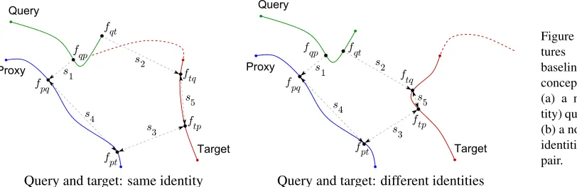
To motivate the meta-features that we propose in this pa-per consider the conceptual illustrations shown in Fig 1. Solid coloured lines depict the range of appearance varia-tion within face sets. Our aim is to estimate the similarity of the query (green) and the set denoted as ‘target’ (red). The face set marked ‘proxy’ is a database face set of a per-son similar in appearance to the ‘target’, as assessed by the baseline similarity measure; for example, the proxies of a
particular target set can be selected as its nearestkpsets in
the database. The dotted red line represents the range of possible appearance of the ‘target’ person which is not ac-tually present in the ‘target’ face set. For the time being the reader may assume that face sets are represented as sets of actual exemplars and the similarity between two sets is given by the similarity between their most similar members – we will explain how the ideas introduced herein can be generalized in the next section.
Both in the case shown in Fig 1(a) and that in Fig 1(b), the baseline similarity measure tells us that ‘query’ is close to ‘proxy’, and of course ‘proxy’ is close to ‘target’ by de-sign i.e. by the former being a proxy in the first place. The difference between the two cases, illustrated conceptually,
lies in the similarity of exemplarsftqandftpi.e. the
exem-plars best matching the query and proxy sets. In particular, the observation that the baseline similarity measure deems the proxy set significantly more similar than the query to the target on the one hand, while both similarities are explained by similar target exemplars, informs us that the divergence in query and proxy appearances from the target are of
dif-ferent natures. Thus, even if similaritiess1,s2, ands3are
the same in Figs 1(a) and 1(b), the information contained in
relationships betweenftq andftp, andfpqandfpttells us
that we should infer different query-target similarities in the two cases. Therefore we introduce what we term transitivity meta-features which we use for the said inference. Given a baseline similarity measure and a triplet consisting of query, target, and proxy sets, the corresponding transitivity
meta-feature v(query,target|proxy)comprises five similarities –
s1 (‘query’ to ‘proxy’ similarity), s2 (‘query’ to ‘target’
similarity),s3(‘proxy’ to ‘target’ similarity),s4(similarity
between the ‘proxy’ exemplar most similar to ‘query’ and
the ‘proxy’ exemplar most similar to ‘target’), ands5
(simi-larity between the ‘target’ exemplar most similar to ‘query’ and the ‘target’ exemplar most similar to ‘proxy’):
(query,target|proxy) =
s1 s2 s3 s4 s5
T (1)
2.3. Non-exemplar based representations
Target Proxy
Query
Target Proxy
Query
[image:3.612.60.466.72.204.2]Query and target: same identity Query and target: different identities
Figure 1. Transitivity
fea-tures extracted using a
baseline set comparison:
conceptual motivation, using (a) a matching (same iden-tity) query-target set pair, and (b) a non-matching (differing identities) query-target set pair.
that the proposed framework is in no way reliant on this representation.
In particular, to make the transition of applying the pro-posed method on the special case in which a face set is rep-resented using a set of directly observed exemplars to the general case in which an arbitrary set representation is em-ployed, we need to explain how the concept of a pair of the
most similar exemplars such as those labelledfqpandfpqin
Fig 1(a), as well as the similarity between them (such as that
betweenfpqandfpt), can be generalized. This is not
diffi-cult – all that is required is a slight reframing of the concept. Instead of seeking the nearest pair of specific exemplars, in the general case we are interested in the pair of the most similar modes of variation captured by the representations of two sets (as measured by the baseline similarity measure of course). We illustrate this idea with a few examples.
If the variation within a set is modelled using a lin-ear subspace and the subspace-to-subspace generalization of the distance from feature space (DFFS) [44] adopted as the (dis)similarity measure between them, the most similar modes of variation between two sets represented using such subspaces are sub-subspaces themselves. These correspond
to different exemplarsfxyin Fig 1 and can be compared
us-ing the DFFS baseline. If, on the other hand, similarity is measured using the maximum correlation between subspace spans as in [6], the most similar modes of variation between two sets are readily extracted as the first pair of the canoni-cal vectors between subspaces [23] and compared using the cosine similarity measure [35]. For manifold-to-manifold
distances such as that of Leeet al. [30] the most similar
modes of variation are simply the nearest pairs of points on two manifolds, with the similarity of two points on the same manifold readily quantified by the geodesic distance between them.
The same ideas are readily applied to any of a variety of set representations and similarity measures described in the literature.
2.4. Learning quasi-transitive similarity
Given a triplet comprising a query, a target, and a proxy data set, our aim now is to infer the similarity between the query and the target using the corresponding transitivity
fea-ture defined in (1). Without loss of generality, let us
quan-tify inter-set similarity with a real number in the range[0,1],
where0 signifies the least and1the greatest possible
sim-ilarity. Then our problem can be stated more formally by
saying that we are seeking a mappingmqts:
mqts:R
5
→[0,1], (2)
with the ideal output ofmqts(v(query,target|proxy))being
0 iff the identities in the query and target sets are different, and 1 iff they are the same. Observe that since we are inter-ested in confidence-based ranking of all sets in a database,
the codomain of mqts is not the set {0,1}, which would
make this a binary classification problem, but rather[0,1]
(a range) which makes it a regression task.
In the types of problem setting in which face recognition is addressed by most of the existing research, obtaining fea-tures for training, at least in principle, is simple. Whether it is verification (1-to-1 matching) or identification (1-to-N matching), the database ‘known’ to the algorithm comprises data which is, it is assumed, correctly partitioned by the identity. The retrieval setting adopted in this work is more challenging in this sense and consequently the learning pro-cess needs to be approached with more care. In particular, as described in Sec 1, we assume that our database is en-tirely unlabelled and that it may contain multiple sets of the same person. We neither know how many individuals there are in the database nor the number of sets of each individual (which can of course vary person to person). Since for any two database sets we cannot know for certain if they belong to the same or different individuals, an obvious corollary is that in the extraction of transitivity features described by (1) both intra-personal and inter-personal training sets may contain incorrect examples.
2.4.1 Extraction of transitivity features for training
(producing differing identities training data). Instead, we describe how training data, albeit corrupted (this issue is dealt with in the next section), can be collected by consider-ing only pairs of sets, that is, all possible database sets and their proxies. We do this for the two baseline set comparison
methods adopted from Wolfet al.[45]: (i)maximum
max-imorum cosine similarity between sets of exemplars [35], and (ii) the maximum correlation between vectors confined to linear subspaces describing within set variability [6, 12].
Exemplar-based baseline Consider a particular database face set (‘reference’) used for training and one of its proxies. To extract training transitivity features which correspond
to same identity query-target comparisons, we selectboth
query and target data from the reference set (i.e. a single video). In particular, we treat all possible pairs of
exem-plars in the reference set as possible pairsfqtandftq.
In-deed, for specific choices of possible query and reference sets, any two appearances may present themselves as the
nearest exemplars in them. The second elements2in the
transitivity feature is then simply given by the similarity be-tween the two exemplars. On the other hand the similarity
s1 between the query and the proxy is given by the
sim-ilarity between the unitary set consisting of the reference
set exemplar treated asfqt and the proxy set. The nearest
proxy exemplar tofqt is of coursefpq. The similarity s3
is simply computed as the similarity between the reference
set and the proxy, which also gives us exemplarsfpt and
ftp, and allows for a straightforward computation ofs4(as
the similarity betweenfpqandfpt) ands5(as the similarity
betweenftqandftp). A single pair of reference and proxy
sets thus gives usnr(nr−1)‘positive’ training transitivity
features, wherenr is the number of faces in the reference
set.
The extraction of training transitivity features which cor-respond to differing identities query-target comparisons is similar. Now we iterate through all exemplar pairs of the
proxy set, taking each pair as fqt and fpq in turn. The
closest target exemplar tofqt becomes ftq, whilefpt and
ftp are determined as before, allowing for all transitivity
feature entries (exemplar similarities) to be computed as in the case of same identity query-target training data extrac-tion. A single pair of reference and proxy sets thus gives us
np(np−1) ‘negative’ training transitivity features, where
npis the number of faces in the proxy set.
It is important to observe that the set of ‘negative’ train-ing transitivity features extracted in the described manner may be corrupt. This is an inherent consequence of the problem setting – since the database is entirely unlabelled we cannot know if the identities of the people in the refer-ence and proxy set are actually different. The proposed pro-cess of training the regressor, described in Sec 2.4.2, takes this into account. Nevertheless, the amount of improve-ment achieved with the proposed method over its baseline
is tied to the proportion of ‘negative’ training data which is incorrect – the improvement inevitably decreases as this proportion is increased. However, if this is so, i.e. if a great proportion of proxies of sets in the database actually repre-sent the same identity as the sets they are proxies to, this by design means that the baseline comparison is very good to start with so no significant improvement can be reason-ably expected. Thus, our method is particularly attractive in challenging conditions in which the baseline classifier does not perform well.
Subspace-based maximum correlation baseline The extraction of training data for this representation is some-what simpler than in the previous case. We again extract transitivity feature training data using only face set pairs (rather than triplets) which are now represented by linear subspaces. To extract training transitivity features which correspond to same identity query-target comparisons, we
iterate through all reference set exemplars as fqt and
ob-tainftq andfpqby projecting them to respectively the
ref-erence and proxy subspaces. Vectorsfptandftpare readily
obtained using the baseline set comparison as the princi-pal vectors of the subspaces corresponding to reference and proxy subspaces. A single pair of reference and proxy sets
thus gives usnr‘positive’ training transitivity features.
The extraction of training transitivity features which correspond to differing identities query-target comparisons proceeds in exactly the same manner, with the difference
that it is proxy set exemplars that are iterated through asfqt
(as before also taken to befqp). A single pair of reference
and proxy sets gives usnr‘positive’ training transitivity
fea-tures, wherenris the number of faces in the reference set,
andnp‘negative’ training transitivity features, wherenpis
the number of faces in the proxy set. A single pair of
ref-erence and proxy sets thus gives usnp ‘negative’ training
transitivity features. The same remarks as before regarding the corruption of the ‘negative’ training set hold here too.
Closing note In Sec 2.1 we remarked that the basic idea behind the proposed method can be seen as complementary to that of MBS [45]. However when the proposed training scheme is considered it can be seen to contain both
con-ceptually similar elementsandcomplementary elements to
MBS. In particular, since the negative training set of quasi-transitivity features is extracted by considering elements of the proxy set as the query, our method learns to discrimi-nate precisely between a person and those individuals most similar to him/her (as in MBS), while exploiting the quasi-transitivity of similarity (complementary to MBS).
2.4.2 Training the predictor
We adopt the use of the ǫ support vector (ǫ-SV)
regres-sion [41]. For comprehensive detail of this regression
relevant to the proposed method. Given training data
{(x1, y1), . . . ,(xl, yl)} ⊂ F ×R, where F is the input
space (in our case this isR5),ǫ-SVR aims to find a
func-tionh(x)which deviates at mostǫfrom its targetsy. As
in other SV-based methods, an implicit mapping of input
data x → Φ(x) is performed by employing a
Mercer-admissible kernel [33]k(xi, xj) which allows for the dot
products between mapped data to be computed in the input space:Φ(xi)·Φ(xj) =k(xi, xj). The functionh(x)of the
form
h(x) =
l
X
i=1
(αi−α∗i)k(xi, x) +b (3)
is then learnt by minimizing
l
X
i=1 l
X
j=1
(αi−α∗i)(αj−α∗j)k(xi, xj)
+ǫ
l
X
i=1
(αi+α∗i)− l
X
i=1
yi(αi−α∗i) (4)
subject to the constraintsPl
i=1(αi−α
∗
i) = 0andαi, α∗i ∈
[0, c]. The parameterccan be seen as penalizing prediction
errors greater thanǫi.e. as balancing the trade-off between
the smoothness ofh(x)and the amount of data predicted
with an error greater thanǫ.
The nature ofǫ-SV regression is particularly well suited
to the problem at hand. Specifically, we train the regres-sor using the value of 1 as the target for same identity transitivity features, and 0 for different identities,
allow-ing for a large prediction error margin of ǫ = 0.4 but
severely penalizing greater errors with c = 1000. The
large penaltyC ensures that it is the outliers in the form
of the wrongly labelled training data that define the bound-ary between the penalized and non-penalized regions of the
high-dimensional space, while the wide marginǫ= 0.4
en-sures that the correctly labelled bulk of the training corpus is pushed away from the boundary towards the desired ex-treme values of 0 and 1. We used the radial basis function kernelk(xi, xj) = exp{−0.2kxi−xjk2}.
2.4.3 Retrieval
Given a query data set we compute its similarity with a target database set by computing the regression-based
es-timatemqts(v(query,target|proxy))using each of target’skp
proxies, and taking the maximum of these and the baseline similarity between the query and the target. Database sets are then ordered by decreasing similarity with respect to the query.
3. Evaluation
In this section we report our evaluation of the proposed method and discuss our findings. We start by describing the data set on which the evaluation was performed, consider the measures used to assess performance, summarize the
0 0.05 0.1 0.15 0.2 0.25 0.3 0.35 0.4 0.45 0.5 0
0.2 0.4 0.6 0.8 1
Nonlinear principal component energy
Cumul
at
ive
probab
ilit
y
[image:5.612.340.510.67.141.2]2nd relative to 1st 3rd relative to 1st
Figure 2. The cumulative distribution function (CDF) of the data energy contained in the 2nd and 3rd nonlinear kernel PCA com-ponents relative to the energy of the 1st component, across sets in the YouTube Faces Database. The variation within sets is strongly dominated by the 1st nonlinear principal component.
Robust samples Original feature space
1D KPCA space
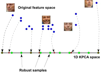
Figure 3. Conceptual illustration of our robust sample selection: (i) original exemplars are projected onto their 1st kernel principal component, (ii) uniform sampling between the extreme projections is performed in the 1D kernel space, and (iii) the obtained samples are re-projected into the original space (step not shown).
0 0.05 0.1 0.15 0.2 0.25 0
0.2 0.4 0.6 0.8 1
Relative error of set−to−set comparisons
Cumul
at
ive
probab
ilit
[image:5.612.339.516.204.330.2]y
Figure 4. CDF of the error introduced by our robust sample selec-tion (10 samples were used) in the exemplar-based set method.
evaluated baseline set representations, distances and their derivatives, and finally present and comment on the results.
3.1. Evaluation data
For evaluation we adopted the YouTube Faces
Database [45] which contains sets of faces extracted from YouTube videos. There are two key reasons which motivated this choice. Firstly, the manner in which this data set was collected and the nature of its contents are representative of the conditions which the present work
targets. In particular, the total amount of data is large
[image:5.612.335.511.394.470.2]for each person in the database. The second reason lies in the reproducibility of results and the ease of comparison with alternatives in the literature – the database has been widely adopted as a standard benchmark and a number of standard face representations are provided ready for use. Full detail can be found in the original publication [45].
3.2. Performance evaluation
As the cornerstone measure of retrieval performance we adopt the average normalized rank (ANR) [19, 37]. In brief, ANR treats each retrieved datum as either matching or not matching the query and computes the average rank of the
former group, normalized to the range[0,1], with the ANR
value of 0 corresponding to the best possible performance (all matching data retrieved before any non-matching) and 1 the worst (all non-matching data retrieved before any matching). Formally:
AN R(n,{r1, . . . , rc}) =
Pc
i=1ri−m
M−m (5)
wherenis the database size,{r1, . . . , rc}the set of retrieval
ranks corresponding to the data of interest (i.e. data
match-ing the query), andmandMrespectively the minimum and
maximum possible values of the sum ofr1, . . . , rc:
m=
c
X
i=1
i= c×(c+ 1)
2 (6)
M =
n
X
i=n+1−c
i=c×2n−c+ 1
2 (7)
In comparison with other common performance mea-sures, such as the receiver operating characteristic (ROC) curve [22], commonly used in verification and identification problems [7], the average normalized rank more directly captures the ultimate aim of a retrieval algorithm.
3.3. Methods
Motivated by the results reported by Wolfet al. which
demonstrate its superiority over a number of alternatives, we adopt the standard local binary pattern (LBP) represen-tation of individual faces [27]. Using LBP we consider two baseline set representations: (i) a set of LBP exemplars, and (ii) a linear LBP subspace, both of which were also
evalu-ated by Wolfet al.The former simply stores all face
exem-plars (i.e. the corresponding LBP vectors), while the latter uses PCA to represent the main modes of the observed ex-emplar variation; previous work suggests that for individual face sets 6-dimensional subspaces produce good results so this is the dimensionality we adopt too.
We adopt two baseline set similarity measures, again mo-tivated by the reports of their good performance in the
ex-isting literature. The first of these is themaximum
maxi-morum(‘max-max’) cosine similarity between sets of ex-emplarsmaxf1∈S1,f2∈S2f1Tf2/kf1k/kf2kwhich in the
ex-periments of Wolfet al.[45] outperformed a number of
al-ternatives including by a large margin the pyramid match
kernel of Graumanand and Darrell [24] and the
locality-constrained linear coding (LLC) of Wanget al.[43]. The
second baseline comparison which we adopt for the com-parison of sets represented as linear subspaces is the alge-braic method based on the maximum correlation between pairs of vectors lying in two subspaces. This method too performed well in past experiments [45, 6]. Thus in sum-mary, our two baseline methods are:
• LBP +maximum maximorumset similarity, and
• LBP + maximum correlation between subspaces.
These are used to establish reference performance. They are then employed in the context of several different ways of applying our idea of quasi-transitivity:
• Simple arithmetic mean-based quasi-transitivity,
• Simple geometric mean-based quasi-transitivity,
• Simple quadratic mean-based quasi-transitivity, and
• Proposed learnt quasi-transitivity (L-QTS).
The first three methods in the list are simple combination rules. In the first of these, the arithmetic mean-based
quasi-transitivity, two set similarity of dissimilarity measuresρQP
(query-proxy) and ρP T (proxy-target) are combined by
computing their arithmetic mean i.e.0.5×(ρQP +ρP T).
Similarly, in the geometric and quadratic mean-based meth-ods quasi-transitivity is attempted by computing
respec-tively√ρQP×ρP T and
p
0.5ρQP2+ 0.5ρP T2. The
pro-posed learnt quasi-transitivity (applied atop of both baseline methods) was evaluated using different numbers of proxy
sets (1–10) and as detailed in Sec 2.4.2,ǫ-SV regression was
learnt using the parameter valuesǫ= 0.4andc= 1000.
3.4. Protocol
We train theǫ-SV regressor using 200 randomly selected
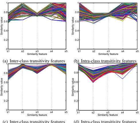
sets and their proxies (which are not necessarily in the ran-dom 200). In principle there is no reason why the entire database would not be used (recall that no labelling or man-ual intervention is used whatsoever) but we found that 200 sets were sufficient to gather sufficient training data. Exam-ples are shown in Fig 6; clear patterns are observable both within positive and negative training sets which differ one from another significantly.
The evaluation of the methods described in the previous section was performed by examining all possible retrievals. In other words, we used every set in our database as the query in turn and evaluated the resulting retrieval. To make this feasible we propose a robust sample selection method so as to reduce the computational demands of the otherwise computationally intensive exemplar-based baseline.
0 0.1 0.2 0.3 0.4 0.5 0.6 0.7 0.8 0.9 1 0 0.1 0.2 0.3 0.4 0.5 0.6 0.7 0.8 0.9 1
Average normalised rank
Cumul at ive probab ilit y dist ribut io n Baseline Simple arithmetic mean Simple geometric mean Simple quadratic mean Proposed L−QTS, 10 proxies
(a) Exemplar b/line, var. methods
0 0.1 0.2 0.3 0.4 0.5 0.6 0.7 0.8 0.9 1 0 0.1 0.2 0.3 0.4 0.5 0.6 0.7 0.8 0.9 1
Average normalised rank
Cumul at ive probab ilit y dist ribut io n Baseline
Proposed L−QTS, 1 proxy Proposed L−QTS, 2 proxies Proposed L−QTS, 5 proxies Proposed L−QTS, 10 proxies
(b) Exemplar b/line, proposed
0 0.1 0.2 0.3 0.4 0.5 0.6 0.7 0.8 0.9 1 0 0.1 0.2 0.3 0.4 0.5 0.6 0.7 0.8 0.9 1
Average normalised rank
Cumul at ive probab ilit y dist ribut io n Baseline Simple arithmetic mean Simple geometric mean Simple quadratic mean Proposed L−QTS, 10 proxies
(c) Subspace b/line, var. methods
0 0.1 0.2 0.3 0.4 0.5 0.6 0.7 0.8 0.9 1 0 0.1 0.2 0.3 0.4 0.5 0.6 0.7 0.8 0.9 1
Average normalised rank
Cumul at ive probab ilit y dist ribut io n Baseline
Proposed L−QTS, 1 proxy Proposed L−QTS, 2 proxies Proposed L−QTS, 5 proxies Proposed L−QTS, 10 proxies
[image:7.612.64.546.55.151.2](d) Subspace b/line, proposed
Figure 5. CDF of the average normalized rank obtained using the exemplar-based (a,b) and subspace-based (c,d) methods. (a,c) Comparison of the respective baseline approach, the three simple quasi-transitivity estimation methods, and the proposed learnt quasi-transitivity. (b,d) Comparison of the respective baseline approach and the corresponding proposed method for different numbers of proxies.
nonlinear, the appearance variation is mostly approximately smooth – this is sometimes somewhat loosely stated as the face appearance being constrained to a nonlinear appear-ance manifold [32, 44]. That being said, the range of
ap-pearance variation of a person’s face within asinglevideo
typically covers only a portion of the entirety of possible variation. It is a simple yet important observation that even within this range of appearance the underlying manifold is not uniformly sampled, e.g. a person may spend more time in a specific pose than in others. One consequence is that while largely redundant face exemplars of the densely sampled portions of the manifold add little new information about the appearance of the person’s face, they can dramat-ically increase the computational cost of set-based compar-isons. This is the case for example for face set-based com-parisons which utilize all sample pairs comcom-parisons such as
those based on themaximum maximorumsimilarity (i.e. all
pairs maximum similarity) [18] or themaximum minimorum
distance (a variation of the Hausdorff distance [42]). More worryingly, if a sample voting scheme is used [45], redun-dant exemplars can unduly affect the result even though they carry little additional information.
We overcome both of the problems described above by employing a robust sample selection scheme. Our starting point is the observation that although the intrinsic dimen-sionality of the entire face manifold is estimated to be in the range 15–22 [31], the appearance variation exhibited in a typical video clip is typically dominated by a single fac-tor such as face yaw changes; the plot in Fig 2 corroborates this. Led by this insight we employ kernel principal com-ponent analysis (KPCA) [39] to project the original face ex-emplars onto their dominant nonlinear principal component, uniformly sample the resulting 1D space between the two projections of the two most extreme exemplars, and finally project them back into the original space. The process is illustrated in Fig 3. The plot in Fig 4 demonstrates that the proposed sample selection does not greatly affect inter-set similarities; a computational improvement of over 2.5 or-ders of magnitude (approximately 330 times) was achieved.
3.5. Results and discussion
The main set of results of our experiments is summarized in the plots in Fig 5(a) and 5(c) which show the cumulative
s1 s2 s3 s4 s5
0 0.2 0.4 0.6 0.8 1 Similarity feature S imilarit y value
(a) Inter-class transitivity features
s1 s2 s3 s4 s5
0 0.2 0.4 0.6 0.8 1 Similarity feature S imilarit y value
(b) Intra-class transitivity features
s1 s2 s3 s4 s5
0 0.2 0.4 0.6 0.8 1 Similarity feature S imilarit y value
(c) Inter-class transitivity features
s1 s2 s3 s4 s5 0 0.2 0.4 0.6 0.8 1 Similarity feature S imilarit y value
(d) Intra-class transitivity features
Figure 6. Training data for the exemplar-based (a,b) and subspace-based (c, d) experiments, in the form of intra-class and inter-class transitivity features shown using parallel coordinates.
densities of the ANR achieved for the two baseline methods and different quasi-transitivity approaches. Firstly note that the two baseline methods performed approximately equally well, which is consistent with the previous reports in the
literature [45]. The three simple attempts at exploiting
[image:7.612.308.552.194.408.2]1 2 3 4 5 0
0.2 0.4 0.6 0.8 1
Number of retrievable in−class videos
P
roport
io
n
of
re
tri
evals
wit
h
>0
mat
ch
in
top
100
Empirical (proposed L−QTS) Empirical (baseline) Predicted (L−QTS) Predicted (baseline)
1 2 3 4 5
0 0.5 1 1.5
Number of retrievable in−class videos
Mean
number
of
target
set
s
ret
rieved
in
top
100
Empirical (proposed L−QTS) Empirical (baseline) Predicted (L−QTS) Predicted (baseline)
[image:8.612.57.422.71.198.2]Match prob. w/in rank-100 Match num. w/in rank-100
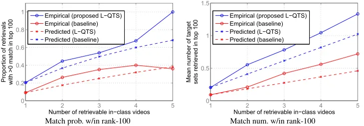
Figure 7. Rank-100: (a) prob-ability of a correct match be-ing retrieved, and (b) number of correct matches retrieved, vs. number of matches in the database.
produced bad results (i.e. high ANR) – for both baselines our method achieved ANR lower than 0.5 for over 98% of retrievals. In contrast, the 98% quantile of the baseline methods corresponds to the ANR values of 0.92 and 0.88 for the exemplar and subspace-based methods.
The effect of the number of proxies is summarized in Figs 5(b) and 5(d). For both baselines performance im-provement is immediately apparent even using a single proxy per set. Interestingly, while in the case of the exem-plar baseline the performance gradually improves up until
kp = 5, staying approximately steady thereafter, the
im-provement using the subspace-based baseline is much more dramatic and reaches its peak (on par with the peak of the
exemplar baseline) for kp = 1 already (ANR plots for
differentkp are virtually indistinguishable). Although we
are not sure of the exact mechanism that explains this be-haviour, it does appear to be linked to the inherent properties of the subspace-based baseline which is additionally sup-ported by the observation that the within-class variability of the corresponding training meta-features is significantly smaller than for the exemplar-based baseline; see Fig 6.
Let us next turn our attention to the plot in Fig 7(a). It shows the proportion of retrievals which result in at least one correct match being retrieved in the top 100 ranked sets as a function of the total number of target sets in
the database which correctly match the query. Plotted
as solid blue and red lines are the results obtained using the proposed method (with 10 neighbours used as quasi-transitivity proxies) atop of the exemplar-based baseline, and the baseline itself (as expected from Fig 5, the results for the subspace-based method are similar and are thus not included to avoid unnecessary repetition). The plots also show predictions based on the methods’ performances for queries in which only a single correct match is present in the entire database. Specifically, starting from the estimate
of the probabilityp1,100of a correct match being retrieved
in the top 100 ranked sets using queries where only a sin-gle correct match is possible, if different correct matches
are ranked independently whenkcorrect matches exist, the
probability of at least a single correct match being retrieved
in the top 100 is approximately1−(1−p1,100)k. Since
the greatest number of admissible queries (591 individuals
in the database have only a single set; these were not mean-ingful queries for performance evaluation), approximately
48%, hask = 1this is a reasonable estimate to base the
prediction on.
Fig 7(a) reveals interesting insight into the performance of the proposed method. Specifically, note that unlike the empirical plot of the baseline, the empirical plot of the pro-posed method grows faster with the number of retrievable sets than the corresponding prediction. This means that the independence assumption underlying the prediction does not hold well, supporting the premise that quasi-transitivity of similarity can be used to improve the retrieval of sets poorly retrieved by the baseline by propagating information from similarly looking individuals or sets of the same per-son which are acquired in less challenging conditions.
Lastly Fig 7(b) shows the average number of correct matches retrieved in the top 100 ranked sets as a function of the total number of target sets in the database which correctly match the query. As before the plots also show the corresponding predictions based on the methods’ per-formances for queries in which only a single correct match
is present in the entire database. Starting from n1,100 the
average number of correct matches retrieved in the top 100 ranked sets using queries where only a single correct match is possible, if different correct matches are ranked
independently when kcorrect matches exist, the expected
number of correct matches in the top 100 is approximately
k ×n1,100. The improvement effected by the proposed
method is again consistent and significant.
4. Summary and conclusions
We introduced a novel framework for improving the per-formance of retrieval algorithms on large and highly hetero-geneous face sets acquired in uncontrolled conditions. In sharp contrast to the previous work, the proposed method
learns to benefit from inter-personalsimilarity using what
References
[1] O. Arandjelovi´c. Unfolding a face: from singular to
mani-fold.In Proc. Asian Conference on Computer Vision, 3:203–
213, 2009.
[2] O. Arandjelovi´c. Colour invariants under a non-linear photo-metric camera model and their application to face recognition
from video.Pattern Recognition, 45(7):2499–2509, 2012.
[3] O. Arandjelovi´c. Computationally efficient application of the generic shape-illumination invariant to face recognition from
video.Pattern Recognition, 45(1):92–103, 2012.
[4] O. Arandjelovi´c. Gradient edge map features for
frontal face recognition under extreme illumination changes.
In Proc. British Machine Vision Conference, 2012. DOI: 10.5244/C.26.12.
[5] O. Arandjelovi´c. Making the most of the self-quotient
im-age in face recognition. In Proc. IEEE International
Con-ference on Automatic Face and Gesture Recognition, 2013. DOI: 10.1109/FG.2013.6553708.
[6] O. Arandjelovi´c. Discriminative extended canonical
corre-lation analysis for pattern set matching. Machine Learning,
94(3):353–370, 2014.
[7] O. Arandjelovi´c. A framework for improving the
per-formance of verification algorithms with a low false
pos-itive rate requirement and limited training data. In Proc.
IEEE/IAPR International Joint Conference on Biometrics, 2014. DOI: 10.1109/BTAS.2014.6996275.
[8] O. Arandjelovi´c. Hallucinating optimal high-dimensional
subspaces.Pattern Recognition, 47(8):2662–2672, 2014.
[9] O. Arandjelovi´c and R. Cipolla. Automatic cast listing in
feature-length films with anisotropic manifold space. In
Proc. IEEE Conference on Computer Vision and Pattern Recognition, 2:1513–1520, 2006.
[10] O. Arandjelovi´c and R. Cipolla. Face set classification using
maximally probable mutual modes. In Proc. IAPR
Interna-tional Conference on Pattern Recognition, pages 511–514, 2006.
[11] O. Arandjelovi´c and R. Cipolla. Achieving robust face recog-nition from video by combining a weak photometric model
and a learnt generic face invariant. Pattern Recognition,
46(1):9–23, 2013.
[12] O. Arandjelovi´c, R. I. Hammoud, and R. Cipolla. Thermal and reflectance based personal identification methodology
in challenging variable illuminations. Pattern Recognition,
43(5):1801–1813, 2010.
[13] K. Assaleh, T. Shanableh, and K. Abuqaaud. Combined
fea-tures for face recognition in surveillance conditions.
Ad-vances in Neural Information Processing Systems, pages 503–514, 2014.
[14] T. L. Berg, A. C. Berg, J. Edwards, M. Maire, R. White, Y. W. Teh, E. Learned-Miller, and D. A. Forsyth. Names and faces
in the news. In Proc. IEEE Conference on Computer Vision
and Pattern Recognition, 2:848–854, 2004.
[15] K. Bowyer, K. Chang, P. Flynn, and X. Chen. Face recogni-tion using 2-D, 3-D, and infrared: is multimodal better than
multisample? In Proc. IEEE, 94(11):2000–2012, 2006.
[16] Y. Cao, Q. Ying and P. Li. Similarity metric learning for
face recognition.In Proc. IEEE International Conference on
Computer Vision, pages 2408–2415, 2013.
[17] R. Chellappa, P. Sinha, and P. J. Phillips. Face recognition
by computers and humans.Computer, 43(2):46–55, 2010.
[18] T. Cour, B. Sapp, A. Nagle, and B. Taskar. Talking pictures: Temporal grouping and dialog-supervised person
recogni-tion. In Proc. IEEE Conference on Computer Vision and
Pattern Recognition, 2010.
[19] T. Deselaers, D. Keysers, and H. Ney. Classification error rate for quantitative evaluation of content-based image
re-trieval systems. In Proc. IAPR International Conference on
Pattern Recognition, 2:505–508, 2004.
[20] M. Everingham, J. Sivic, and A. Zisserman. Taking the bite
out of automatic naming of characters in TV video. Image
and Vision Computing, 27(5):545–559, 2009.
[21] M. Everingham and A. Zisserman. Identifying individuals in video by combining generative and discriminative head mod-els. In Proc. IEEE International Conference on Computer Vision, 2005.
[22] T. Fawcett. An introduction to ROC analysis.Pattern
Recog-nition Letters, pages 861–874, 2006.
[23] K. Fukumizu, F. Bach, and A. Gretton. Consistency of kernel
canonical correlation analysis.Journal of Machine Learning
Research, 8:361–383, 2007.
[24] K. Grauman and T. Darrell. The pyramid match kernel:
Dis-criminative classification with sets of image features. In
Proc. IEEE International Conference on Computer Vision, 2:1458–1465, 2005.
[25] A. Hadid and M. Pietik¨ainen. Combining appearance and
motion for face and gender recognition from videos.Pattern
Recognition, 42(11):2818–2827, 2009.
[26] Y. Haitovsky. A note on the maximization ofR¯2
.The Amer-ican Statistician, 23(1):20–21, 1969.
[27] M. Heikkil¨a, M. Pietik¨ainen, and C. Schmid. Description of
interest regions with local binary patterns. Pattern
Recogni-tion, 42(3):425–436, 2009.
[28] H. Hu. Face recognition with image sets using locally
Grass-mannian discriminant analysis. IEEE Transactions on
Cir-cuits and Systems for Video Technology, 24(9):1461–1474, 2014.
[29] G. B. Huang, M. Ramesh, T. Berg, and E. Learned-Miller. Labeled faces in the wild: A database for studying face recognition in unconstrained environments. Technical Re-port 07–49, University of Massachusetts, Amherst, October 2007.
[30] K. Lee, M. Ho, J. Yang, and D. Kriegman. Acquiring linear
subspaces for face recognition under variable lighting.IEEE
Transactions on Pattern Analysis and Machine Intelligence, 27(5):684–698, 2005.
[31] M. B. Lewis. Face-space-R: towards a unified account of
face recognition.Visual Cognition, 11(1):29–69, 2004.
[32] Y. M. Lui and J. R. Beveridge. Grassmann registration
mani-folds for face recognition.In Proc. European Conference on
Computer Vision, 2:44–57, 2008.
[33] J. Mercer. Functions of positive and negative type and their
connection with the theory of integral equations.
[34] B. Moghaddam and A. Pentland. Probabilistic visual
learn-ing for object representation. IEEE Transactions on Pattern
Analysis and Machine Intelligence, 19(7):696–710, 1997. [35] H. V. Nguyen and L. Bai. Cosine similarity metric learning
for face verification.In Proc. Asian Conference on Computer
Vision, 2:709–720, 2010.
[36] D. Ozkan and P. Duygulu. A graph based approach for
nam-ing faces in news photos.In Proc. IEEE Conference on
Com-puter Vision and Pattern Recognition, 2:1477–1482, 2006.
[37] G. Salton and M. J. McGill. Introduction to Modern
Infor-mation Retrieval.McGraw Hill, New York, 1983.
[38] B. Sch¨olkopf and A. Smola. Learning with kernels. MIT
Press, Cambridge, MA, 2002.
[39] B. Sch¨olkopf, A. Smola, and K. M¨uller.Advances in Kernel
Methods – SV Learning, chapter Kernel principal component analysis., pages 327–352. MIT Press, Cambridge, MA, 1999. [40] J. Sivic, M. Everingham, and A. Zisserman. Person spotting:
video shot retrieval for face sets.In Proc. IEEE International
Conference on Image and Video Retrieval, pages 226–236, 2005.
[41] V. Vapnik. The Nature of Statistical Learning Theory.
Springer-Verlag, 1995.
[42] E. P. Vivek and N. Sudha. Robust hausdorff distance measure
for face recognition. Pattern Recognition, 40(2):431–442,
2007.
[43] J. Wang, J. Yang, K. Yu, F. Lv, T. Huang, and Y. Gong. Locality-constrained linear coding for image classification.
In Proc. IEEE Conference on Computer Vision and Pattern Recognition, pages 3360–3367, 2010.
[44] R. Wang, S. Shan, X. Chen, and W. Gao. Manifold-manifold distance with application to face recognition based on image set. In Proc. IEEE Conference on Computer Vision and Pat-tern Recognition, pages 1–8, 2008.
[45] L. Wolf, T. Hassner, and I. Maoz. Face recognition in
uncon-strained videos with matched background similarity.In Proc.
IEEE Conference on Computer Vision and Pattern
Recogni-tion, pages 529–534, 2011.
[46] M. Yang, D. Kriegman, and N. Ahuja. Detecting faces in
images: A survey. IEEE Transactions on Pattern Analysis
and Machine Intelligence, 24(1):34–58, 2002.
[47] Q. Yin, X. Tang, and J. Sun. An associate-predict model for
face recognition. In Proc. IEEE Conference on Computer
Vision and Pattern Recognition, pages 497–504, 2011. [48] W. Zhao, R. Chellappa, P. J. Phillips, and A. Rosenfeld. Face
recognition: A literature survey. ACM Computing Surveys,