C
2014. The American Astronomical Society. All rights reserved. Printed in the U.S.A.
REDSHIFT EVOLUTION OF THE DYNAMICAL PROPERTIES OF MASSIVE GALAXIES FROM SDSS-III/BOSS
Alessandra Beifiori1,2,3, Daniel Thomas2,4, Claudia Maraston2, Oliver Steele2, Karen L. Masters2,4, Janine Pforr2,5, Roberto P. Saglia1,3, Ralf Bender1,3, Rita Tojeiro2, Yan-Mei Chen6,7, Adam Bolton8, Joel R. Brownstein8,
Jonas Johansson2,9, Alexie Leauthaud10, Robert C. Nichol2,4, Donald P. Schneider11,12, Robert Senger1, Ramin Skibba13, David Wake6,14, Kaike Pan15, Stephanie Snedden15, Dmitry Bizyaev15, Howard Brewington15,
Viktor Malanushenko15, Elena Malanushenko15, Daniel Oravetz15, Audrey Simmons15, Alaina Shelden15, and Garrett Ebelke15
1Max-Planck-Institut f¨ur Extraterrestrische Physik, Giessenbachstraße, D-85748 Garching, Germany;[email protected] 2Institute of Cosmology and Gravitation, University of Portsmouth, Dennis Sciama Building, Burnaby Road, Portsmouth PO1 3FX, UK
3Universit¨ats-Sternwarte M¨unchen, Scheinerstrasse 1, D-81679 M¨unchen, Germany 4SEPNET, South East Physics Network
5NOAO, 950 N. Cherry Avenue, Tucson, AZ 85719, USA
6Department of Astronomy, University of Wisconsin-Madison, 475 N. Charter Street, Madison, WI 53706, USA 7Department of Astronomy, Nanjing University, Nanjing 210093, China
8Department of Physics and Astronomy, University of Utah, Salt Lake City, UT 84112, USA 9Max-Planck Institut f¨ur Astrophysik, Karl-Schwarzschild Straße 1, D-85748 Garching, Germany 10Institute for the Physics and Mathematics of the Universe (IPMU), The University of Tokyo, Chiba 277-8582, Japan
11Department of Astronomy and Astrophysics, The Pennsylvania State University, University Park, PA 16802, USA 12Institute for Gravitation and the Cosmos, The Pennsylvania State University, University Park, PA 16802, USA
13Department of Physics, Center for Astrophysics and Space Sciences, University of California, 9500 Gilman Drive, San Diego, CA 92093, USA 14Department of Physical Sciences, The Open University, Milton Keynes MK7 6AA, UK
15Apache Point Observatory, P.O. Box 59, Sunspot, NM 88349-0059, USA
Received 2013 November 20; accepted 2014 May 6; published 2014 June 18
ABSTRACT
We study the redshift evolution of the dynamical properties of∼180,000 massive galaxies from SDSS-III/BOSS combined with a local early-type galaxy sample from SDSS-II in the redshift range 0.1 z 0.6. The typical stellar mass of this sample isM ∼2×10¹¹M. We analyze the evolution of the galaxy parameters effective
radius, stellar velocity dispersion, and the dynamical to stellar mass ratio with redshift. As the effective radii of BOSS galaxies at these redshifts are not well resolved in the Sloan Digital Sky Survey (SDSS) imaging we calibrate
the SDSS size measurements withHubble Space Telescope/COSMOS photometry for a sub-sample of galaxies.
We further apply a correction for progenitor bias to build a sample which consists of a coeval, passively evolving population. Systematic errors due to size correction and the calculation of dynamical mass are assessed through Monte Carlo simulations. At fixed stellar or dynamical mass, we find moderate evolution in galaxy size and stellar velocity dispersion, in agreement with previous studies. We show that this results in a decrease of the dynamical to stellar mass ratio with redshift at >2σ significance. By combining our sample with high-redshift literature data, we find that this evolution of the dynamical to stellar mass ratio continues beyondz∼0.7 up toz >2 as Mdyn/M ∼(1 +z)−0.30±0.12, further strengthening the evidence for an increase ofMdyn/M with cosmic time.
This result is in line with recent predictions from galaxy formation simulations based on minor merger driven mass growth, in which the dark matter fraction within the half-light radius increases with cosmic time.
Key words: galaxies: elliptical and lenticular, cD – galaxies: evolution – galaxies: formation – galaxies: high-redshift – galaxies: kinematics and dynamics
Online-only material:color figures
1. INTRODUCTION
Early-type galaxies play an important role in observational studies of galaxy formation and evolution. Tight empirical cor-relations between the observed dynamical and stellar popula-tion properties of early-type galaxies have been derived that set useful constraints to their formation histories. These are correla-tions between size (effective radius,Re), surface brightness and
stellar velocity dispersion (σe), i.e., the fundamental plane (FP;
Dressler et al.1987; Djorgovski & Davis1987; Bender et al.
1992,1993), the stellar mass plane (Hyde & Bernardi2009b;
Auger et al. 2010a), the fundamental manifold of galaxies
(Zaritsky et al.2008), as well as correlations between galaxy color and stellar population age and metal abundance with galaxy mass (see review by Renzini2006).
Such scaling relations represent a powerful phenomenologi-cal tool to study the co-evolution of baryonic and dark matter in galaxies. The latter has been studied extensively for the lo-cal galaxy population. The tightness of the FP has been used to constrain stellar population variations or dark matter content in galaxies (Renzini & Ciotti1993) or to study non-homology (Ciotti et al.1996). Gerhard et al. (2001) studied the dynami-cal properties and dark halo sdynami-caling relations of giant elliptidynami-cal galaxies and found that the tilt of the FP is best explained by a stellar population effect and not by an increasing dark matter fraction with luminosity.
using self-consistent models (see Cappellari et al. 2013a for a review). Other studies based on Sloan Digital Sky Survey (SDSS; York et al.2000) data came to the conclusion that there is an excess over the predictions of stellar population models with a fixed IMF which are luminosity dependent (Padmanabhan et al.2004; Hyde & Bernardi2009a,2009b).
These conclusions have recently been revised in Cappellari
et al. (2013b) by means of a large number of axysimmetric
dynamical models including different representations of dark matter halos reporting a variation of IMF slope with galaxy mass. In fact, as highlighted by Thomas et al. (2011), for instance, dark matter fraction and IMF are highly degenerate. They studied a sample of Coma galaxies and their detailed decomposition into luminous and dark matter reveals that for low-mass galaxies there is a good agreement between dynamical masses with dark matter halo and lensing results (galaxies with
a σ ∼ 200 km s−1 are consistent with a Kroupa IMF). For
higher-mass galaxies (σ >200 km s−1), the disagreement can be due to either a non constant IMF (Kroupa IMF under-predicts luminous dynamical masses for galaxies atσ ∼ 300 km s−1) or to a dark matter component which follows the light (see also Wegner et al.2012).
A promising complementary approach to detailed studies of local galaxies for breaking the degeneracy between dark matter fraction and IMF is to study the evolution of fundamental plane, dynamical and stellar population properties of galaxies
with look-back time (Bender et al.1998; van Dokkum et al.
1998; Treu et al. 2005; Jørgensen et al. 2006; Saglia et al.
2010; Houghton et al.2012; Bezanson et al.2013a). Moreover, dark matter fractions can also be studied in samples of lensed galaxies at different redshifts (see Bolton et al.2012ausing data from both the Sloan Lens ACS sample, SLACS; Bolton et al.
2006,2008, and the BOSS Emission line Lens Survey, BELLS; Brownstein et al.2012).
A large number of such investigations have been performed in recent years, analyzing the redshift evolution of galaxy sizes (e.g., Daddi et al. 2005; Trujillo et al. 2006a, 2006b, 2007; Longhetti et al.2007; Zirm et al.2007; Toft et al. 2007; van Dokkum et al.2008; Buitrago et al.2008; Cimatti et al.2008; Franx et al.2008; Bernardi2009; Damjanov et al.2009; Saracco et al.2009; Bezanson et al. 2009; Mancini et al.2009,2010; Valentinuzzi et al.2010a; Carrasco et al.2010; Szomoru et al.
2012; Newman et al.2012; Saracco et al.2014) and dynamical properties of galaxies (van der Wel et al.2005,2008; Cenarro & Trujillo2009; Cappellari et al.2009; van Dokkum et al.2009; Newman et al.2010; Onodera et al.2010; Saglia et al.2010; van de Sande et al.2011,2013; Toft et al.2012; Onodera et al.
2012; Damjanov et al.2013; Belli et al.2014). The bottom line is that galaxy sizes appear to decrease (at fixed stellar mass) and stellar velocity dispersions increase (at fixed stellar mass) with increasing look-back time. Some of these conclusions are still controversial, however. Tiret et al. (2011), for example, argue that the size evolution disappears when one homogenizes literature data sets by measuring the stellar mass with the same method and provides accurate estimates of the sizes to prevent systematic effects in the Re measurements of low
signal-to-noise ratio (S/N) high-zcompact galaxies (Mancini et al.2009). Mancini et al. (2010) also report evidence for galaxies as large as local ones at redshift higher than 1.4 suggesting that not all high-zgalaxies are compact. Moreover, the effect depends on the photometric band and on whether galaxies have young or old light-weighted ages and if they reside in clusters or field (see Valentinuzzi et al.2010bfor clusters and Poggianti et al.
2013for field studies; see also Trujillo et al.2011for a different opinion).
So far, galaxies in the distant universe (look-back times of a few billion years and above) have not been studied at the same statistical level as local galaxies. The new data set from the Baryon Oscillation Spectroscopic Survey (BOSS; Dawson et al.2013) as part of the Sloan Digital Sky Survey-III (SDSS-III; Eisenstein et al.2011) provides the opportunity to investigate the dynamical and stellar population properties of a galaxy sample of unprecedented size up to redshifts z ∼ 0.7. The survey is currently obtaining spectroscopic data for nearly 1.5 million massive galaxies at redshifts between 0.2 and 0.7, hence up to look-back times of∼6 Gyr. The combination of this sample with local early-type galaxies from SDSS-I/II allows us to make a statistically significant link between local galaxy properties and higher redshift observations. This is the main aim of the present paper.
The paper is organized as follows. The galaxy sample is de-scribed in Section 2. Photometric, kinematic, and dynamical properties are presented in Section3, as well as the calibration technique for measuring the effective radii based on a
sub-sample of galaxies with Hubble Space Telescope(HST)
pho-tometry and the correction for progenitor bias. The results are presented in Section 4and discussed in Section 5. The paper concludes with Section6.
Throughout the paper, we assume the following cosmology withH0 =71.9 km s−1Mpc−1,Ω
m =0.258, andΩΛ =0.742
following the cosmology used for the stellar mass determination of BOSS galaxies in DR9 (Maraston et al.2013).
2. DATA
We use the galaxy sample from SDSS-III/BOSS covering a
redshift range 0.2 z 0.7. To leverage our study on the redshift evolution, we combine this sample with a local sample of massive galaxies atz∼0.1 drawn from SDSS-II.
2.1. Main Galaxy Sample from SDSS-III/BOSS
Data are taken from the SDSS-III/BOSS Data Release Nine
(DR9, Ahn et al. 2012). BOSS (Dawson et al. 2013; Smee
et al. 2013), one of the four surveys of SDSS-III (Eisenstein et al.2011), is taking spectra for 1.5 million luminous massive galaxies with the aim of measuring the cosmic distance scale and the expansion rate of the Universe using the Baryonic Acoustic Oscillations (BAO) scale (Anderson et al.2012). Data are taken with an upgraded version of the multi-object spectrograph on
the SDSS telescope (Gunn et al.2006). BOSS galaxy targets
are selected from the SDSS ugriz imaging (Fukugita et al.
1996; Gunn et al.1998; Stoughton et al.2002), including new imaging part of DR8 mapping the southern Galactic hemisphere. A series of color cuts have been used to select targets for BOSS spectroscopy (Dawson et al. 2013). The selection criteria are designed to identify a sample of luminous and massive galaxies with an approximately uniform distribution of stellar masses following the Luminous Red Galaxy (LRG; Eisenstein et al.
redshifts. These two population are well separated in the (g−r) and (r−i) colors diagram (Masters et al.2011).
To extract a working set of objects from the entire BOSS sample, we matched galaxies from different catalogs of stellar velocity dispersions and stellar masses described in the
fol-lowing sections using the keywords PLATE, MJD, FIBERID
that uniquely determine a single observation of a single ob-ject. The final merged catalog comprises 491,954 galaxies that are included in DR9. We selected objects from the LOWZ and
CMASS samples (BOSS_TARGET1 = Target flags) with a
good platequality (PLATEQUALITY = ‘‘good’’), with
ob-ject class “galaxy” (class_noqso = GALAXY), with
high-confidence redshifts (ZWARNING_NQSO = 0), and for which we have a unique set of objects in the case of duplicate observations (SPECPRIMARY = 1).
The final sample we will analyze comprises∼180,000 objects (37% of the original sample) obtained after applying some additional redshift cuts and quality cuts to stellar velocity dispersions and stellar masses that we will discuss in Section3.
2.2. Local Galaxy Sample from SDSS-II
In order to connect our BOSS galaxies to the local galaxy population, we use a sample of galaxies from the SDSS Data Release Seventh (DR7; Abazajian et al.2009). We select early-type galaxies following Hyde & Bernardi (2009a). Galaxies had to be well fitted by a de Vaucouleurs profile in thegandrbands (fracDeV_g=1fracDeV_r=1), with an early-type-like spec-trum (eClass<0), extinction-correctedr-band de Vaucouleurs magnitudes in the range 14.5<deVMag_r<17.5 (this results in a tighter limit compared to that of the SDSS Main Galaxy sample; see details in Hyde & Bernardi2009a), measured stel-lar velocity dispersion in DR7velDisp>0, and with an axis ratio in the rband of b/a > 0.6, to be more likely pressure supported. As described in Hyde & Bernardi (2009a), the DR7
b/a distribution shows two distinct populations separated by this axis-ratio value with a 20% of low-luminosity objects at
b/a <0.6.16This retains∼123,500 DR7 objects.
Bernardi et al. (2010) did a detailed comparison of different methods to select early types in the literature (morphologically based, colors, or structural parameters-based methods), showing that Hyde & Bernardi (2009a) cuts give similar results to other methods but is more efficient in discriminating elliptical galaxies from spirals, which is important in our analysis.
We select galaxies with zWarning = 0 and apply some
constraints on the errors of the parameters: errors onRe<70%,
errors on the axis ratios 0<errb/a<1, errors inσ <30%. Only
galaxies with stellar velocity dispersion of 70< σ <550 km s−1 were selected, following the BOSS cuts.
3. GALAXY PROPERTIES
The primary aim of this work is to study the redshift evolution of the dynamical properties of BOSS galaxies. Stellar masses are taken from Maraston et al. (2013) and stellar velocity dispersions from Thomas et al. (2013). Both of these quantities are included
16 We do not apply this cut in our BOSS sample becauseb/afrom the SDSS imaging could be highly unreliable. In fact, we do not find the same clear separation in theb/adistribution of BOSS galaxies. Also, the BOSSb/a distribution looks different probably due to the large uncertainties onb/afrom SDSS imaging. However, we assess the typical percentage of galaxies which should have ab/a <0.6 by using the sub-sample of BOSS galaxies with COSMOS photometry (see Section3.2.2for details) and find that∼22% of galaxies have ab/a <0.6, which is consistent with Masters et al. (2011) findings. Finally, the choice of this cut does not affect appreciably our results.
in the DR9 data release. We used a sub-sample of 240 galaxies
with additionalHST/COSMOS photometry and BOSS spectra
(Masters et al. 2011) to derive a calibration for galaxy sizes from DR8. In the following sections, we describe the galaxy parameters in more detail. In Section3.4, we describe how the effective radii and stellar velocity dispersion are combined to derive virial masses.
The redshifts used in our analysis are those extracted from
DR9 asz_noqsowith formal 1σerror given byz_err_noqso
(outputs of the BOSS pipeline as described in Bolton et al.
2012b; Dawson et al. 2013). Redshifts are successfully
deter-mined for ∼98% of CMASS galaxies (Anderson et al. 2012,
their Table 1). Errors in the measured redshift are less than about 0.0002 (∼60 km s−1). BOSS observed a few galaxies at z > 0.7 andz <0.2. In our analysis, we focus on the redshift range 0.2 z 0.7 and therefore excluded all the galaxies outside this redshift range. This cut retains 90% of the galaxies (444,118 objects).
3.1. Stellar Mass
We use the stellar massesMfrom Maraston et al. (2013) as
published in the DR9 data release.17These masses are derived through broadband spectral energy distribution (SED) fitting of model stellar populations on SDSSu, g, r, i, zmodelMag mag-nitudes from DR8, scaled to thei-bandcmodelMagmagnitude. The BOSS spectroscopic redshift is used to constrain the fits. We note that the DR9 data release also provides alternative mass estimates from Chen et al. (2012; see Maraston et al.2013for discussion).
Maraston et al. (2013) use different types of templates to derive stellar masses; passive models, star-forming models or a mix, chosen so as to match the galaxy expected galaxy type, based on a color cut, in BOSS.18 In this paper we used stellar masses obtained with the passive template that is a mix of old populations with a spread in metallicity and which was found to reproduce well the colors of luminous red galaxies at redshift 0.4 to 0.7 (Maraston et al.2009). This maximally old and passive
LRG template minimizes the risk of underestimatingMwhich
is the typical effect that occurs when one determines stellar masses from light (Maraston et al.2010; Pforr et al.2012).
We adopt the stellar masses derived from the median of the probability distribution function (PDF). Typical uncertainties on
Mare<0.1 dex, independently of redshift (see Maraston et al.
2013for details).
The Portsmouth stellar mass pipeline described in Maraston et al. (2013) provides stellar masses using various types of configurations, i.e., Kroupa (2001) or Salpeter (1955) IMF, passive (Maraston et al.2009) or star-forming (Maraston et al.
2006) models, and considering or not the mass loss in the stellar evolution. The subset of calculations used here adopt a Kroupa IMF. As is well known, a Salpeter IMF produces systematically larger stellar masses by about a factor 1.6 (Maraston 2005; Bolzonella et al.2010). Systematic uncertainties are mainly due to the choice of the IMF (∼0.2 dex).
We removed galaxies for whichM was not properly
deter-mined due to unreliable values of redshift and photometry issues. This cut retains 387,590 galaxies (79% of the full sample).
17 Stellar masses have been derived for galaxies with non-zero photometry in
i-bandmodelmag_i > 0.0,z_err_noqso 0andz_noqso > z_err_noqso.
3.2. Size
The photometric data used in this paper were derived using
the SDSS-III DR8 pipeline (Aihara et al. 2011). One of the
main updates performed in DR8 compared to Stoughton et al. (2002) is the correction for sky levels (in particular for extended galaxies) which past studies found to be overestimated (Bernardi et al. 2007; Lauer et al. 2007; Guo et al. 2009). This issue has also been addressed in detail in Blanton et al. (2011). SDSS effective radii are adopted from the DR8 catalog. In this section we describe this measurement and its calibration with
COSMOS/HSTimaging.
3.2.1. SDSS DR8 Effective Radii
Effective radii are estimated using seeing-corrected de Vau-couleurs effective radii (deVRad) and the associated errors (deVRadErr; of the order of∼5%–25% depending on redshift). Those values correspond to the effective radius along the semi-major axis derived on elliptical aperture.
BOSS galaxies are often not well resolved in SDSS imaging.
The average seeing of the SDSS survey is 1.05 from the
PSF_FWHMin the i-band (lower and upper percentile of 0.88 to 1.24), which is better than in previous data releases due to the repeated images taken during the survey (see Ross et al.
2011; Masters et al.2011). The median effective radius of BOSS galaxies (after having applied the previous cuts on the sample) is 1.24 (upper and lower percentile 2.12 and 0.72, respectively). As a consequence, seeing effects will affect size measurements (see Saglia et al.1993,1997; Bernardi et al.2003), which we need to correct for. To develop a seeing correction we compare SDSS galaxy radii with measurements based on high-resolution
HST/COSMOS imaging (Section3.2.3).
The surface brightness models used by pipeline to obtain galaxy sizes are relatively simple (single parameter fits, i.e., ex-ponential or de Vaucouleurs profiles); a more complex model is not feasible for this analysis because of the limitation of the image resolution. We tested this conclusion and found that per-forming S´ersic fits on BOSS images yields strong degeneracies between effective radius and S´ersic index, preventing robust es-timate of effective radii. We eses-timate SDSS circularized radii asRe,circ =Re×q1/2 whereReis the semi-major axis of the
half-light ellipse andq =b/ais the axis ratio which is part of the DR8 catalog.
The effective radii should, in principle, be referred to a fixed rest-frame wavelength to account for the fact that early types have color gradients, so on average their optical radii are larger in bluer bands and at higherz this effect will make the sizes larger (see Bernardi et al.2003; Hyde & Bernardi 2009a for discussions). We did not apply any correction for this trend, because uncertainties of the size calibration (∼10%–25%) are larger than the typical variation in size measured in different filters (from 4% to 10%; Bernardi et al.2003; Hyde & Bernardi
2009a). In Section4.1we describe the average effect this could have on the size evolution studies.
Effective radii were converted to physical radii using the code of Hogg (1999) which presents the scale conversion between arcsec and kiloparsec for our given cosmology. Hereafter, we will use the notationpipeline Reto represent SDSS effective radii in kiloparsecs. We further remove from the catalogs galaxies with unreliable values ofReand their errors. This cut retains ∼370,000 objects.
3.2.2. COSMOS Effective Radii
Masters et al. (2011) constructed a sub-sample of 240
BOSS galaxies withHST/COSMOS imaging (Koekemoer et al.
2007; Leauthaud et al. 2007). This sample was used to cal-ibrate the SDSS DR8 radii part of the CMASS sample. We adopted the effective radii from the publicZurich Structure & Morphology Catalog v1.019 (Scarlata et al. 2007;
Sargent et al. 2007) derived from I-band (F814W) ACS
im-ages. Effective radii are available from this catalog for 224 of the 240 objects.
The catalog contains galaxy structural parameters derived
from a two-dimensional decomposition using theGIM2Dcode
(Galaxy Image 2D; Simard 1998) on the ACS/HST images
as deep as IAB ∼ 22.5 (Sargent et al. 2007). We used the
seeing-corrected effective radiiR_GIM2Dresulted from the one component S´ersic fit, of the form
I(r)=Ie10[−bn((r/Re,)
1/n−1)]
, (1)
whereIeis the effective intensity, and the constantbnis defined in terms of the shape parameternand is chosen so thatRe,encloses
half of the total luminosity and it is measured in arcsec. The quantitybncan be well approximated bybn=0.868n−0.142
(Caon et al.1993). TheZurich Structure & Morphology
Catalog v1.0 contains two values of the effective radius from GIM2D, R_GIM2D and R_0P5_GIM2D which correspond to the point-spread function (PSF)-corrected effective radii. The choice of one of the two is purely arbitrary and they show a negligible median difference of 0.001 (withR_GIM2Dbeing smaller thanR_0P5_GIM2D). The catalog gives the uncertainties on effective radii as 99% confidence lower and upper error onR_GIM2D(LE_R_GIM2D,UE_R_GIM2D, respectively). Those errors are<1% ofR_GIM2D, much smaller than the errors inRe
from SDSS photometry (∼15% in the COSMOS/BOSS
sub-sample).
Sizes are converted to circularized effective radii Re,serc
following the procedure described in Saglia et al. (2010)20
which calculates the half-light radius obtained from the classical curve of growth analysis of the intrinsic S´ersic profile. The
procedure requires R_GIM2D, S´ersic indexSERSIC_N_GIM2D,
and axis ratio q = b/a, where a, b are the semi-major and
minor axis of the half-light ellipse, and q = 1 −, where
is the ellipticity of the object ELL_GIM2D. Here we use
a different parameterization than in Section 3.2.1 because
we have additional information from the S´ersic fit (the two parameterization would give consistent results for a wide range ofq).
We did not apply any correction to account for the fact that rest-frame wavelengths are different at different redshifts
using only i-band data because this sample is only used
for calibration purposes, and uncertainties due to the size calibration we derive using COSMOS radii are much larger than the wavelength variation at the redshifts considered (see Section3.2.1). Moreover, COSMOS has just one filter available for those galaxies. COSMOS radii were converted to kiloparsecs in the same way as SDSS radii using the code of Hogg (1999). Hereafter, we will use the notationCOSMOSRe,Serto represent
COSMOS effective radii in kiloparsecs.
19 Available athttp://irsa.ipac.caltech.edu/data/COSMOS/datasets.html. 20 The code is available at
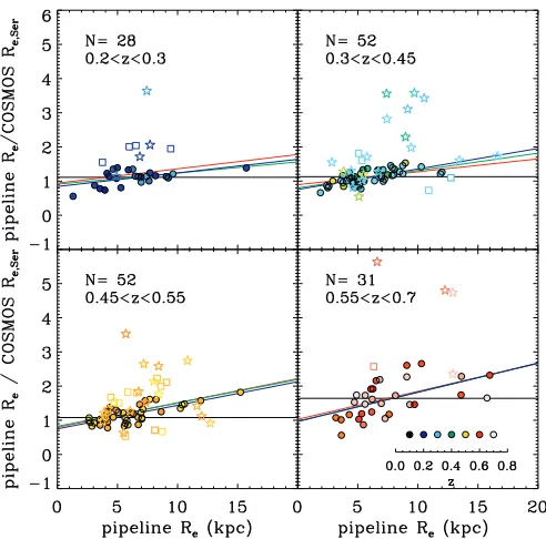
Figure 1.Ratio between pipelineRefrom SDSS DR8 and COSMOSRe,Seras a function of pipelineRe. Points are coded as a function of redshift (0.2z0.3, 0.3 < z 0.45, 0.45 < z < 0.55, and 0.55 z 0.7). Different lines represent different fitting procedures: the red line is a linear fit, the green line is a linear fit with one 2σclip, the blue line is iterative 2σclipping, the horizontal black line is the single offset. Circles are the points that have been used in the fit and open squares are points discarded in the iterative sigma clipping. Open stars are multiple systems inHSTimaging which are unresolved in the SDSS images (Masters et al.2011). Labels in each panel give the number of galaxies used in the fit including objects discarded in the iterative 2σclipping (multiple systems are not included in this number).
(A color version of this figure is available in the online journal.)
3.2.3. Comparison SDSS versus COSMOS
A significant fraction (23%) of BOSS galaxies with HST
imaging are unresolved multiple systems in SDSS imaging (Masters et al.2011). To derive an accurate calibration, we ex-cluded these unresolved multiple systems from our analysis (44 galaxies) using the public catalog of Masters et al. (2011).21The
redshift range we wish to study is 0.2z0.7, and we dis-carded 4 additional galaxies at higher redshifts and 13 atz <0.2. This leaves us a sample of 163 galaxies. COSMOS redshifts are adopted, as not all of these objects (158 out of 163) have BOSS redshifts (this will not change our results, because the median difference between COSMOS and BOSS redshifts is negligible, 7.21×10⁻⁶). We do not correct for PSF variations in the SDSS
imaging, because the PSF is reasonably stable and the effect is negligible compared to the overall correction derived here.
Figure 1 shows the ratio between SDSS and COSMOS
effective radii as a function of SDSS effective radius for four redshift bins. The ratio is around 1.1, and SDSS radii can be overestimated by up to a factor two. The discrepancy between SDSS and COSMOS radii increases with increasing SDSS radius (see also Masters et al.2011). Masters et al. (2011)22 found that a single offset was reproducing their data in which they compared the ratio SDSS over COSMOS radii as a function of COSMOS radii. In this work, we compare the ratio of SDSS over COSMOS radii as a function of SDSS radii to derive a
21 Available athttp://www.icg.port.ac.uk/∼mastersk/BOSSmorphologies/. 22 Masters et al. (2011) estimated the size correction only for the CMASS sample and used major axis radii.
Table 1
Size Correction for the Four Redshift Bins
zRange N a b c
0.2z0.3 24 0.84±0.11 0.04±0.01 0.29±0.04 0.3< z0.45 48 0.75±0.06 0.06±0.01 0.19±0.02 0.45< z <0.55 41 0.75±0.04 0.07±0.01 0.32±0.03 0.55z0.7 30 0.97±0.17 0.08±0.02 0.49±0.06
Notes.A correlation of the formRe,pipeline/Re,COSMOS,Ser=a+b(Re,pipeline)
is assumed.Nis the number of points used in the fit after iterative 2σclipping. Uncertainties on each parameter are 1σerrors. The rms scattercis derived as deviation of the data about the fits considering also objects discarded by the 2σclipping.
correction for the full BOSS sample. As is to be expected, there is also some redshift dependence, in the sense that SDSS radii overestimate most the true radii at higher redshifts. Also, as expected, the scatter of the relationships increases with redshift owing to the decrease in SDSS imaging quality.
The size calibration could be affected by the larger uncertain-ties in the SDSS effective radii due to the higher than typical
sky background (60%–70%) of SDSS images in the COSMOS
field (Masters et al.2011; Mandelbaum et al.2012; on the other hand, seeing is smaller than typical of 10%–15%) which could give relations between SDSS and COSMOS radii not universal for the full BOSS sample.
We performed fits to these relationships in the four redshift bins independently. We tested for linear correlations applying different levels of sigma clipping in the linear fits: no sigma clipping, red line in Figure1; just one 2σ clipping, green line in Figure1; and an iterative 2σ clipping, blue line in Figure1
with a maximum of three iterations.
We fitted a linear relation of the form Re,pipeline/
Re,COSMOS,Ser = a+b(Re,pipeline). The best-fit quantitiesaand b, the number of galaxies used in the fit after the sigma clip-ping, the scatter of the relationsc(which include objects dis-carded by the 2σ-clipping), and their associated errors obtained as 1σ uncertainties for each redshift bin are listed in Table1. The least-square fits were performed using theMPFITalgorithm (Markwardt2009) under theIDL23 environment. Fits with and without sigma clipping are consistent within the errors.
The slope of the relation increases slightly with redshift as to be expected. The scatter about the relation is comparable in the first three redshift bins, while the last redshift bin shows a considerably higher scatter (see Table1;c=0.49±0.06). For this reason, we will only use the first three redshift bins in the analysis.
We tested the significance of the fits through an F-test by comparing the resultingχ2values for free and fixed slope fits accounting for the number of degrees of freedom, and find a maximum probability of no relation to be∼2%, which confirms the statistical validity of our fits. The final fits we adopt for the radius correction in each redshift bin are the linear fits with iterative 2σ clipping (blue lines) because they give corrections with a smaller scatter compared to other fits (of 6%–30%). The open squares in Figure1are those galaxies that were discarded in the sigma clipping. Open stars represent unresolved multiple systems not considered in the fits.
We additionally searched for correlations of the effective radius with several other DR8 structural parameters like axis
ratio b/a, fracdev, and the difference between fiber2mag
23 Interactive Data Language is distributed by Exelis Visual Information Solutions. It is available from
[image:5.612.317.570.75.136.2](a) (b) (c)
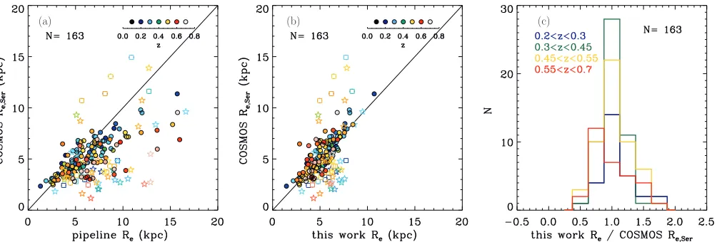
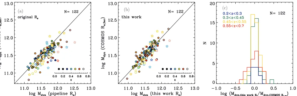
Figure 2.Left panel: COSMOSRe,Seras a function of pipeline SDSSRecoded in terms of redshift. Middle panel: COSMOSRe,Seras a function of rescaled SDSS
Re(used in the present work) coded in terms of redshift. Symbols are as in Figure1. Right panel: distribution of the ratio between SDSS rescaledReand COSMOS Re,Serfor the four redshift bins in Figure1. Histograms contain also discarded objects but not multiple systems. Legends in each panel give the number of galaxies used in the derivation of the size correction including objects discarded in the iterative 2σclipping (multiple systems are not included in this number).
(A color version of this figure is available in the online journal.)
andmodelmagwith the aim at finding the best parameter space for the radius correction. None of these parameters helped improving the radius correction.
The size correction we derive here accounts also for the fact that galaxies in our sample could have been better described by a S´ersic profile rather than a de Vaucouleurs, therefore we should consider our calibrated sizes as “S´ersic-like.”
3.2.4. Radius Calibration
Figure2, panel (b), shows the final corrected radii that are obtained using the fits of Figure1. For comparison, panel (a) shows the uncorrected radii. Panel (c) presents the distribution of the ratio between the SDSS and COSMOS radii in various redshift bins after the correction. The radii agree well at all redshifts after the correction has been applied. More specifically, the median ratio between our rescaledReand COSMOSRe,Ser
is 1.02 (upper and lower quartile 1.34 and 0.86 and mean 1.10) for 0.2 z 0.3, 0.98 (upper and lower quartile 1.15 and 0.85 and mean 1.01) for 0.3< z0.45, 1.01 (upper and lower quartile 1.31 and 0.84 and mean 1.05) for 0.45 < z < 0.55, and 0.99 (upper and lower quartile 1.41 and 0.73 and mean 1.02) for 0.55z0.7. Median values of the distributions in each redshift are compatible within±1σ/N1/2, whereNis the number of objects. Typical errors on rescaled radii range from 0.7 kpc atz∼0.2 to 1.0 kpc atz∼0.7 and median radii range from 5.34 to 4.28 kpc, mode 4.73 to 3.48 kpc, in this redshift range. If we did not apply the size correction, we would have larger radii (median sizes range from 5.72 kpc atz∼0.25 to 5.40 kpc atz∼0.55, 6.51 kpc atz∼0.65, mode from 5.00 to 4.00 kpc and 5.00 atz∼0.65).
Filled circles in Figure2are those galaxies that were used in the previous section to derive the calibration. Open squares are those objects that were discarded in the iterative 2σ clipping. Open stars are the unresolved multiple systems discarded from the calibration. Most of the multiples are strong outliers in these plots and they would have been discarded during the sigma clipping fit.
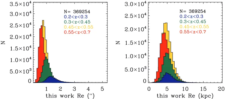
Figure3shows the resulting distributions of galaxy effective radii (in both arcseconds and kiloparsecs) for the final sample of 369,254 galaxies in the various redshift bins. The size distribution can be described by a log-normal function (as
the typical size distribution at low redshift; Shen et al. 2003; Bernardi et al.2003) but with different peaks of the distributions suggesting a variation of typical sizes with z. In Section 4, we present our results using both the corrected SDSS size and pipeline sizes (which we circularized using SDSS axis ratio for this purpose).
3.2.5. Systematic Errors
The systematics in the error budget have been assessed through Monte Carlo simulations which account for uncertain-ties in both parametersaandbof the fit. The average errors vary with redshift in a non-linear fashion. The errors are∼0.6 kpc at
z∼0.25,∼0.2 kpc atz∼0.55, and∼0.6 kpc atz∼0.65. We additionally include in our Monte Carlo simulations the impact of unresolved multiple systems, which have
systemati-cally overestimated sizes. By using the COSMOS/BOSS
sub-sample, we can estimate that those correspond to the∼6% of the galaxies in this sample (see left panel of Figure13). The sizes of the two components which are resolved in the COSMOS imag-ing (and unresolved in the SDSS imagimag-ing) allow us to assess the contribution of unresolved multiple systems in our analy-sis, which seems to be negligible compared to other systematic uncertainties (see AppendixBfor details).
More detail on the Monte Carlo simulations are given also in Section4, where we discuss the impact on the final science analysis.
3.3. Stellar Velocity Dispersion
Stellar velocity dispersions (σ) are taken from the Portsmouth Spectroscopic pipeline described in Thomas et al. (2013), also available in DR9. Briefly, stellar kinematics are derived by means of the Penalized Pixel-Fitting method pPXF (Cappellari & Emsellem2004) in spectra in which emission lines are fit-ted with Gaussian templates by using the GANDALF code (Sarzi et al.2006). The stellar population models of Maraston & Str¨omb¨ack (2011) have been adopted to fit the stellar contin-uum. These are based on a hybrid model between MILES stellar library (S´anchez-Bl´azquez et al.2006) and theoretical spectra at bluer wavelengths from UVBLUE (Rodr´ıguez-Merino et al.
Figure 3.Histogram of the effective radii derived in this work (after size correction), in arcseconds (left panel) and kiloparsecs (right panel) for various redshift bins as color-coded in Figure2.
(A color version of this figure is available in the online journal.)
therefore needed to be only slightly downgraded to match the
BOSS spectral resolution (R ∼1800–2000 at 5000 Å, 2.78 Å
−2.50 Å FWHM). Stellar velocity dispersions have been
mea-sured in the typical rest-frame wavelength range 4500–6500 Å most suitable for stellar kinematics analysis due to the presence of strong absorption features (Bender1990; Bender et al.1994). Stellar velocity dispersions from the Portsmouth Spectro-scopic pipeline agree within a few percent with other DR9 measurements ofσ by Bolton et al. (2012b) and Chen et al. (2012; see Thomas et al. 2013 for a detailed comparison of the systematic offsets between methods). Thomas et al. (2013) show that the typical error distribution on theσ measurements for BOSS galaxies peaks at 14%, and 93% of the measurements have an error below 30%. We therefore selected objects with an error inσbelow 30% for the present study to be as inclusive as possible while still maintaining an acceptable accuracy in ve-locity dispersion (large errors are due to the low S/N of BOSS spectra, mean∼4.4 fromS_N median, which is sufficient to measure velocity dispersions; Thomas et al.2013). This cut is not as tight as is generally applied but it allows us not to be affected by biases due to sample selection (for example, a com-mon tighter cut with a relative error<10% would discard most of the lowσgalaxies at high redshift). Thomas et al. (2013) also show thatσ determinations show no bias with S/N. Errors on
σeslightly vary with redshift, from 12 km s−1 atz∼ 0.25 to
39 km s−1atz∼0.65.
Besides the cut in relative error below 30%, we further restrict
our sample to values of 70 σ 550 km s−1. We discard
velocity dispersions below 70 km s−1 because of the limit in instrumental resolution of the BOSS spectrograph, and velocity
dispersions above 550 km s−1 to exclude contamination by
potential multiple systems (Bernardi et al.2003,2006,2008). The final number of galaxies that survive these additional cuts in velocity dispersion is∼370,000, which is 75% of the original sample.
The stellar velocity dispersions from BOSS spectroscopy (σap) are measurements within the 2 diameter aperture of
the BOSS fiber. Therefore, we applied an aperture correction to translate the BOSS velocity dispersions to the aperture corresponding to the effective radius using the relation of Cappellari et al. (2006) derived from the integral field data of the SAURON sample
σe=σap×(rap/Re,)0.066 (2)
in which σe is the stellar velocity dispersion withinRe,, and
rap = 1 is the radius of the BOSS fiber.Re, is taken from
the rescaled effective radii converted to arcsecond. The relation of Cappellari et al. (2006) is consistent with that of Mehlert et al. (2003, slope=0.06) and slightly steeper but in agreement within the errors with older determinations by Jorgensen et al. (1995, slope=0.04).
Aperture corrections depend on galaxy profile and systematic evolution in the light profile of galaxies could affect the stellar velocity dispersion, as well as this rescaling factor could change from local SAURON galaxies to the higher redshift BOSS galaxies. However, we expect this effect to be negligible as the aperture corrections are small (maximum 3% at higher redshift) because the fiber diameter is close to the typical effective radius of galaxies at the redshifts studied here (see Figure3). Typical uncertainties after the aperture correction range from 5% to 16% ofσe(13 to 39 km s−1).
3.3.1. Systematic Errors
We performed Monte Carlo simulations to estimate system-atic errors on the aperture correction due to the size calibration (see Section3.2.4), and have found them to be small. On av-erage σe changes by ∼1.5 km s−1, which is well below the
measurements errors.
3.4. Dynamical Mass
Following Beifiori et al. (2012), we estimate dynamical
galaxy mass from the effective radius and velocity dispersion within the effective radius using the virial mass estimator as
Mdyn=βdyn(n)Reσe2/G, (3)
whereGis the gravitational constant andβdynis a dimensionless
constant that depends on galaxy structure, often adopted as
βdyn=5.0±0.1 for local galaxies; see Cappellari et al. (2006).
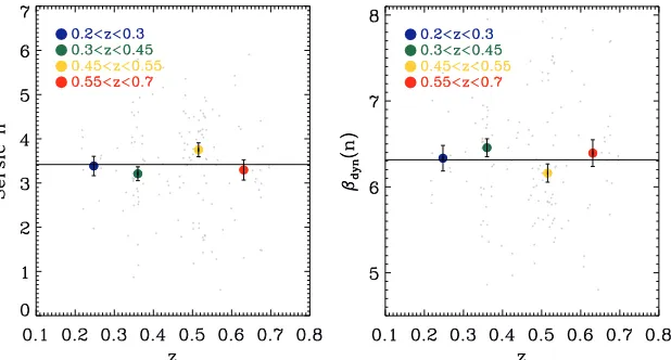
Figure 4.S´ersic indices (left panel) andβdynparameters (right panel; see Equation (3)) of the COSMOS/HSTsample for various redshift bins as color-coded in Figure2. Colored symbols with error bars are the medians. The continuous line is the median value. The total number of objects is 150.
(A color version of this figure is available in the online journal.)
As we are mostly interested in the latter, the main conclusions of this work will not be affected. As an additional check
we therefore compared the Mdyn/M derived here with those
measured for local galaxies from more sophisticated dynamical modeling in and find good agreement (see Section4.3). Still, it should be emphasized that any change in dynamical mass found here reflects a change of dynamical mass within 1Re.
3.4.1. Dependence on Structural Parameters
The appropriate value ofβdyn is actually a function of the
S´ersic shape indexn(Trujillo et al.2004; Cappellari et al.2006). Taylor et al. (2010) showed that dynamical masses and stellar masses correlate well when the structure of the galaxy is taken into account (see also Section3.4.5). They find that dynamical masses estimated with the homology assumption exhibit resid-ual trends with galaxy structure properties, so they introduce a structure-corrected dynamical mass adopting a constantβdyn
that is S´ersic index dependent (Bertin et al.2002). Note that the virial mass estimator of Cappellari et al. (2006) (Equation (3)) has been calibrated on dynamical masses from Schwarzschild modeling where no assumption about homology is made.
For our sample of BOSS galaxies, we cannot make any statements in this respect since SDSS images do not have the necessary angular resolution to perform S´ersic fits. However, we can expect this effect to be negligible, as the BOSS galaxy sample is restricted to massive galaxies in a relatively narrow mass range (Maraston et al.2013) and limited redshift range so that variations of the S´ersic index will be minimal. Moreover, the fact that our size calibration is based on S´ersic Re from
COSMOS, allows us to account for possible differences between de Vaucouleurs profiles and S´ersic profiles resulting in a “S´ersic-like” calibrated radii.
We verify this assumption with the COSMOS sub-sample for
which S´ersic indices are available. The Zurich Structure
& Morphology Catalog v1.0also contains values of galaxy S´ersic index,n. This allows us, for this sub-sample, to account for the variation of the parameterβdyn withnand encapsulate
the effects of galaxy structure onMdyn(by assuming a constant βdyn for all galaxies, Equation (3) implicitly assumes that all
galaxies are homologous).
We estimateβdyn(n) following the analytic expression
be-tweenβdyn(n) and the S´ersic index (Equation (20) of Cappellari et al. 2006), which is theoretically derived for spherical and
isotropic models with a S´ersic profile for different values ofn (Bertin et al.2002; see also Taylor et al.2010for a discussion of its importance on the SDSS sample).
Figure4, right panel, shows the dependence of theβdyn(n)
parameter on redshift for each galaxy in the sub-sample (gray points). Colored circles are the medianβdyn(n) for each redshift bin. We find that the medianβdyn(n) is∼6.3 for all redshifts bins
(see continuous line in Figure4, right panel). This is larger than the local values of 5 generally adopted, and yields systematically higher masses by∼20%. The reason is the relatively low S´ersic indices (between 3.38 and 3.30 atz∼0.25 orz∼0.6, as shown in Figure4, left panel) for the COSMOS sample, compared to typical S´ersic indices for local galaxies.
The key point illustrated by Figure4, however, is that both n andβdyn(n) do not evolve with redshift. As we focus in the redshift evolution and not absolute values for dynamical mass, the present study is not affected by a systematic offset inβdyn. We will useMdynderived using a medianβdyn = 6.3, which
is the median value βdyn derived using the BOSS/COSMOS
photometry.
3.4.2. Dependence on Aperture
The dynamical mass obtained using the virial mass estimator
(see Section 3.4) is based on stellar kinematics within an
aperture of 1 effective radius and scaled to total dynamical mass via Equation (3). This quantity is compared with thetotal stellar mass from Maraston et al. (2013) based oncmodelMag magnitudes. Hence both dynamical and stellar masses aretotal masses, which ensures a consistent comparison.
Still, the total dynamical mass is derived from observations within the effective radius, while the stellar mass comes from the total stellar light. We explore therefore the possible presence of a systematic effect from the different apertures in which kinematics and stellar populations have been measured. To
this end we compareM derived frommodelmag(rescaled to
i-band cmodelmag) andM from aperture magnitudes within
Re (rescaled to i-band cmodelmag). This test is presented in
AppendixA.
In brief, the difference between the two sets of masses is
∼0.08 dex. The stellar masses measured from SED fitting within
1 Re are higher by this amount, because of the higher M/L
(a) (b) (c)
Figure 5.Left panel: dynamical masses derived using the original SDSSReassuming a constantβdyn =6.3 vs. dynamical masses derived using COSMOSRe,Ser adopting a variableβdynbased on the S´ersic index. Symbols are as in Figure1. Middle panel: same as left panel but using rescaled SDSSReadopted in the present study. Right panel: distribution of the ratio of dynamical masses from rescaled SDSSReand COSMOSRe,Serfor the four redshift bins of Figure1. Legends in each panel give the number of galaxies used in the derivation of the size correction including objects discarded in the iterative 2σclipping (multiple systems are not included in this number).
(A color version of this figure is available in the online journal.)
reassuring to verify that this systematic difference is relatively small. Most importantly, the offset is independent of redshift (see AppendixA). Hence, the science analysis of this work is not affected, because we study redshift dependence and do not focus on absolute ratios between dynamical and stellar masses. We also note that the dynamical to stellar mass ratio is always larger than 0.08 dex in our redshift range, henceMdoes never exceed Mdynensuring physically meaningful solutions throughout.
3.4.3. Dependence on Rotation
The possible presence of unresolved rotation is another com-plication that could affect our mass estimates from Equation (3). van der Marel & van Dokkum (2007) have measured increased rotational support atz ∼ 0.5 and argue that data at different redshifts can be affected by rotation, with a stronger impact on low-σ galaxies, which are more rotationally supported than
galaxies at highσ. As our BOSS sample consists of massive
galaxies in a relatively small mass range (Maraston et al.2013), however, we expect this effect to be negligible.
3.4.4. Dependence on Galaxy Type
Finally, in deriving Mdyn with Equation (3), we implicitly
assume that the measured value of σe is dominated by the
bulge component. For late-type galaxies, we expect that the disc contribution toσeresults in a broader distribution ofMdyn,
since theσemay not represent the actual dynamical state of those
galaxies which is dominated by rotation (see Section3.4.3) as well as theβdynparameter we used could not be appropriate for
late-type galaxies with low S´ersic index. As shown in Masters et al. (2011), however, the majority of BOSS galaxies (74%± 6%) have early-type morphology and the remaining later types are bulge dominated, hence this effect will be negligible. We tested this assumption by only considering early-type galaxies for the CMASS sample using the morphological cut (g−i)>
2.35 by Masters et al. (2011). We compared dynamical masses
derived with COSMOS Re and adopting βdyn based on the
S´ersic index and dynamical masses withRederived in this work
and found a good agreement between early types and the full
COSMOS/BOSS sub-samples, with a scatter around the
one-to-one relation consistent within the errors (∼0.14 dex).
3.4.5. Calibrated Virial Masses for the COSMOS Sub-sample
As an additional test, we compare our virial mass estimates based on the re-scaled effective radii with virial masses derived directly from the COSMOS effective radii, the result is shown in Figure5. The left panel shows the comparison between virial
masses derived using COSMOSReand theuncorrectedSDSS
Re. As expected, there is a clear offset to higher virial masses
from SDSS imaging because of the overestimation of galaxy radii.
The re-scaled radius of this work remedies this problem. The middle panel of Figure5shows the comparison between virial
masses derived using COSMOS Re, and adopting a variable
βdyn based on the S´ersic index (see Section 3.4.1) and the correctedSDSS Re of the present work (by using a constant βdyn=6.3 as described in Section3.4.1). Mass estimates agree
well at all redshifts with a scatter of∼0.14 dex, which is well within the errors. The right panel presents the distribution of the logarithmic ratio between COSMOS and SDSS masses after correction. The distribution is symmetric around zero for all redshift bins with a maximum deviation of∼0.5 dex.
3.4.6. Random and Systematic Errors
The final errors in Mdyn are a combination of uncertainties
in σe (which account for the aperture scaling of σ), Re, the
statistical uncertainties due to the rescaling factor of Re, and βdyn. This results in median random errors of ∼0.15 dex
depending on redshift (from 0.08 dex at z = 0.25 to 0.18
dex at z = 0.65). Based on Monte Carlo simulations, we
estimate median systematic errors due to the size calibration (see Section3.2.4) and uncertainty ofβdyn(n) to be∼0.04 dex.
3.5. Local SDSS-II Early-type Galaxy Sample
We combine the SDSS-III/BOSS sample described above
with a local sample of massive galaxies at z ∼ 0.1 drawn
from SDSS-II. The galaxy properties of this local sample are presented in the following sections.
3.5.1. Stellar Mass
prescription of Maraston et al. (2013) with passive templates
(the LRG model by Maraston et al.2009 mentioned earlier).
We homogenize the stellar mass distribution by selecting a sub-sample that matches the mass distribution of the BOSS sample. We constructed this sub-sample using the stellar mass distribution in the lowest BOSS redshift bin (0.2 < z < 0.3) as reference. For each stellar mass bin, we randomly selected from the local galaxy distribution a number of galaxies equal
to the number of galaxies in the low-z BOSS one. This cut
on the local early-types population retains 12,089 galaxies. A discussion on the impact of the science analysis in this paper from this homogenization is given in AppendixE.
3.5.2. Size
We collect photometry and effective radiiRe from DR8 in
which the correction for the sky over-subtraction of previous re-leases is already implemented (see discussion in Section3.2.1), and no further correction to sizes (see Hyde & Bernardi2009a, for details) has been applied. This is motivated by the fact that we selected galaxies at redshiftz <0.2 that are resolved in the SDSS imaging withRe>FWHM of the PSF (retaining 96% of
the objects).
3.5.3. Stellar Velocity Dispersion
We collect redshift and stellar velocity dispersions from the DR7 catalogs. Thomas et al. (2013) show that their DR7σ are consistent with SDSS pipelineσ at the few percent level (see their Figure 1). The median offset across all the stellar velocity dispersion is∼1%. However, this offset increases toward high stellar velocity dispersions. We can quantify the correct offset to apply to DR7σ looking at Figure 4 of Thomas et al. (2013) where theirσ are compared to Bolton et al. (2012a)σ within BOSS, which is the relevant mass range.24 The offset is 4%, which we correct for in the SDSS-II sample.
We further rescaled stellar velocity dispersions to the value at Re, following the procedure described in Section3.3, accounting
for the fact that DR7 galaxies were observed with a 3aperture. The variation inσe for the aperture correction in local SDSS
galaxies is 2% (σewithin Re on average 2% smaller than the SDSS ones, and median ratio between aperture size andReis ∼0.72).
3.5.4. Dynamical Mass
Dynamical mass is derived from stellar velocity dispersion and size in the same way as for the BOSS sample as described in Section3.4. To ensure internal consistency, we use the same redshift independent parameterβdyn = 6.3 as for the BOSS
sample derived from the BOSS/COSMOS photometry (see
Section3.4.1).
3.6. Correction for Progenitor Bias
BOSS target selection was designed to obtain a nearly uniform stellar mass distribution across the redshift range 0.2 z 0.7. Still, the sample needs to be corrected for effects from progenitor biases (e.g., Valentinuzzi et al.2010b; Saglia et al.2010; Cimatti et al.2012and references therein), as higher-zgalaxies in the sample are not necessarily progenitors of the lower-z galaxies in the sample (see also Tojeiro et al.
2012).
[image:10.612.339.546.53.264.2]24 Bolton et al. (2012a) is the same code that produced the SDSSσ.
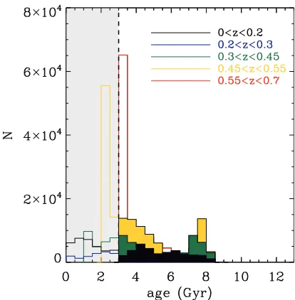
Figure 6.Histograms of the ages for different redshift bins, evolved to the highest redshift bin by subtracting the look-back time, which are used to apply the progenitor-bias cut (see the text for details). Galaxies in the shaded region, i.e., with an age below 3 Gyr, have been discarded.
(A color version of this figure is available in the online journal.)
To correct for the progenitor bias, we compare—in each redshift bin—the galaxy ages from Maraston et al. (2013; one of the products of the SED fit; see Section 3.1) and remove those galaxies from the low-zsample whose ages (evolved to the highest redshift bin by subtracting the look-back time) would be lower than a given age threshold which is the time needed for a typical galaxy to become passive. For each redshift bin, we select galaxies such that their age follows
tg(z)−(tu(z)−tu(z=0.65))>3 Gyr, (4)
wheretgis the age of a galaxy at a give redshift,tuis the age
of the universe at the same redshift, and tu(z = 0.65) is the
age of the universe at the median redshift of the highest-redshift bin. Histograms of the evolved ages for different redshift bins are shown in Figure6. Galaxies in the shaded region have been discarded. As the age threshold we chose 3 Gyr, adopting the age limit used in Maraston et al. (2013)25for calculating stellar
masses (see their Section 3.1 for discussion). This threshold is only slightly larger than the 1.5 Gyr suggested by van Dokkum & Franx (2001).
We considered the highest-redshift bin as a reference and we evolved all other redshift bins including the local SDSS early-type sample. By discarding galaxies with age<3 Gyr, we retain 268,938 galaxies, which correspond to the∼65% of the initial local and BOSS samples as shown in Figure6.
We obtain similar results using the tighter selection criteria described in Cimatti et al. (2012), which select in each redshift bin the galaxies with ages within±1σof the age distribution for each redshift bin accounting for the cosmic time elapsed from one bin to the other. This selection also discards objects at older ages and provides a sample size that is∼54% of the initial one. Poggianti et al. (2013) found that galaxy sizes are correlated to luminosity-weighted ages such that older galaxies will show
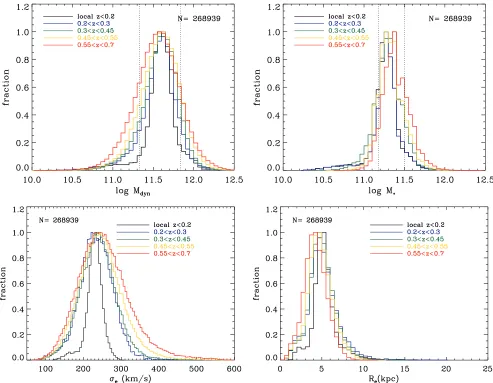
Figure 7.Top panels: distribution ofMdyn(withβdyn=6.3, left panel) andM(right panel) for various redshift bins, normalized to the peak value in each bin. The
BOSS mass distributions are fairly uniform over the redshift range under analysis (see also Figure 10 in Maraston et al.2013). Local early-types from SDSS-II are selected to have the same stellar mass distribution of the lowest BOSS redshift bin. Dotted black lines indicate the±1σof the mass distributions adopted for the present analysis. Bottom left and right panels: distributions in stellar velocity dispersion distribution and effective radius. The progenitor-bias correction has been applied in all cases.
(A color version of this figure is available in the online journal.)
a stronger size evolution, with a stronger effect in clusters than in the field. Our progenitor bias correction minimizes that effect. The distributions ofM,Mdyn,σe, andReof the final sample
after correction for progenitor bias are shown in Figure 7
for various redshift bins. The typical median stellar mass is around logM ∼ 11.28 dex, the median Re ∼ 5.2 kpc, and σe∼231 km s−1.
To study the effect of the progenitor bias correction on the redshift evolution of these quantities, we have performed a re-analysis for a sample without progenitor bias correction presented in AppendixD. It can be seen that generally results are consistent. Most importantly, the evolution ofMdyn/Mis
fairly stable against the progenitor-bias correction, hence the main conclusions of these paper do not critically depend on the progenitor bias correction.
4. RESULTS
In this section, we present the redshift evolution of the galaxy parameters effective radius, velocity dispersion, and dynamical to stellar mass ratio for our final sample of 256,849 SDSS-III/BOSS galaxies and 12,089 local early-type SDSS-II
galaxies with a typical stellar mass of∼2.2×10¹¹ M and a typical dynamical mass of ∼3.9×10¹¹ M
. The results are
presented in Figure 8, where we plot the galaxy parameters
effective radius (left panels), stellar velocity dispersion (middle panels), and dynamical to stellar mass ratio (right panels) as functions of redshift. Shaded regions and contours indicate the number density of galaxies (10 equally-spaced density levels showing the percentage of galaxies compared to the peak value of each plot), and colored circles are the mean for each redshift bin. Fixed intervals in stellar mass and dynamical mass are considered in the top and bottom panels, respectively. They were selected to be within±1σof the mass distributions of Figure7. This allows us to keep a large number of galaxies with similar mass (186,269 and 189,613 galaxies forMandMdynselection
for the full local and BOSS sample, respectively) without being affected by selection effects as a function ofz. A finer division in bothMandMdynwould not change our results.
(a) (b) (c)
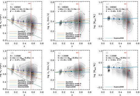
[image:12.612.77.537.55.369.2](d) (e) (f)
Figure 8.Left panels: effective radiusReas a function of redshift. Middle panels: stellar velocity dispersionσeas a function of redshift. Right panels: ratio between dynamical and stellar massMdyn/Mas a function of redshift. Top and bottom panels are for galaxies selected usingMandMdyn, respectively (within±1σof the
mass distributions, total number of galaxies given by the labels). The shaded contour region indicates the full sample after correction for progenitor bias. Contours show 10 equally-spaced density levels showing the percentage of galaxies compared to the peak value of each plot. The colored filled circles are the median values in four redshift bins. The green solid line is a linear fit, the green dashed line is a fit with zero slope for comparison. The black dotted line is a linear fit to the sample if no size correction is applied. Error bars of the median points indicate the 1σuncertainty derived from Monte Carlo simulations. The red continuous lines and arrows indicate the range where we fit our data.
(A color version of this figure is available in the online journal.)
Table 2
Fitting Parameters for the Redshift Evolution of Galaxy Parameters between 0.1z0.55
Parameter M Mdyn
Slope Zero Point Slope Zero Point
Re −0.49±0.26 0.76±0.04 −0.37±0.20 0.73±0.03 σe 0.12±0.02 2.36±0.01 0.18±0.06 2.35±0.01 Mdyn/M −0.48±0.23 0.35±0.03 −0.55±0.17 0.36±0.02
Notes.Uncertainties on each parameter are 1σerrors derived from Monte Carlo simulations. The relation we fitted forRe is logRe = logRe,0+β(1 +z), forσeis logσe =logσe,0+γ(1 +z), and forMdyn/Mis log(Mdyn/M)=
log(Mdyn/M)0+δ(1 +z).
We fit relationships of the form X ∝ (1 +z)slope to all data, but the result does not change significantly by fitting the means. We do not account for galaxies in the last redshift bin atz > 0.55 in the fit because of the larger uncertainty of the radius calibration (see Section3.2.3). The best-fitting values of zero-point, slope, and their associated errors are derived by performing least-squares linear regressions using theMPFIT package. We additionally consider the case where we only fit the zero-point (assuming a zero slope) to test the significance of the derived slopes (dashed lines). We also assess the latter with
a comparison of theχ2values of the two fits for free and fixed slope, accounting for the number of degrees of freedom, using theF-test statistics.
Figure9is a reproduction of Figure8in which the predictions of simulations are shown for comparison. Solid lines in Figure9
are model predictions of Oser et al. (2012), Nipoti et al. (2012) (here we list a couple of models with different stellar-to-halo-mass prescriptions as a function of redshift that those author presented in their work), Hopkins et al. (2009), and Khochfar & Silk (2006) for the evolution of galaxy size and velocity dispersion. The predictions of the redshift evolution ofMdyn/ Mare from Hopkins et al. (2009).
As discussed in the previous sections, the major sources for random and systematic errors are the size correction (Section 3.2) and the calculation of dynamical mass through the virial estimator (Section3.4). To assess random and system-atic errors in the redshift evolution of the galaxy parameters, we perform Monte Carlo simulations perturbing the slopea, the interceptbof the size correction, as well as the structural depen-dent quantityβdyn(n) within their errors. For each redshift bin,
we produced distributions ofa,b, andβdyngenerating random
[image:12.612.41.295.499.567.2](a) (b) (c)
[image:13.612.79.539.55.370.2](d) (e) (f)
Figure 9.Same as Figure8, but with predictions from theoretical models overplotted as solid colored lines for comparison (see labels for references). (A color version of this figure is available in the online journal.)
and9 are estimated through these simulations hence include
both random and systematic errors.
4.1. Evolution of Galaxy Size
The left panel of Figure8shows that galaxy radius decreases with increasing redshift for both choices of mass estimator (top and bottom panels) at 1.5σsignificance. TheF-test between the fits with fixed and free slope yields a probability<25% of the null hypothesis being true (no redshift evolution) for bothM
andMdynselected samples, which supports the significance of
the slope derived here. Qualitatively similar results are obtained when only using the BOSS sample, although uncertainties are
larger and the significance reduced (Appendix C). The size
evolution found in the present work are consistent within the errors with previous determinations in the literature, which are mostly based on data at higher redshifts (e.g., Trujillo et al.
2006a; van Dokkum et al.2008; Cimatti et al.2008; Saracco et al. 2009), but in particular with Saglia et al. (2010), who
studied a similar z range. This agreement further validates
the size correction applied here. Without the latter, we would not detect significant evolution of galaxy sizes (dotted lines in Figure8) in clear contradiction to findings in the literature.
We note again that we did not account for the slightly different mapped rest-frame wavelengths using radii from observed i-band images across all redshifts. This approach is conservative as even smaller sizes would obtained from the rest-frame bluer images at higher redshift (Bernardi et al.2003; Hyde & Bernardi
2009a) with the net effect that we tend to slightly underestimate the size evolution.
In Figure 9 (left panels), we show the comparison of our
results with simulations (solid lines), which show a very wide range of predictions for the slopeβ. The evolution we find is consistent with or slightly milder than the predictions from semi-analytical models or hydrodynamical simulations (Khochfar & Silk2006; Naab et al.2009; Hopkins et al.2009; Nipoti et al.
2012; Oser et al.2012). However, recent work on size evolution suggests that the size evolution atz <1 is much shallower than at high redshifts (Newman et al.2012; Cimatti et al.2012; Nipoti et al.2012), which could explain why we find a milder evolution of the effective radius. This is reinforced by comparsion with the predictions of L´opez-Sanjuan et al. (2012), who studied
close pairs using massive galaxies in COSMOS up to z ∼ 1
and measured the merger fraction and rate from both minor and major mergers. Their models predict a size evolution due to both major and minor mergers, which is in excellent agreement with our results.
4.2. Evolution of Stellar Velocity Dispersion
The middle panels of Figure8show the evolution ofσewith redshift. We detect a mild but significant evolution of stellar velocity dispersion, in the sense thatσeincreases with increasing
redshift at>2σ significance. Again, theF-test between the fits with fixed and free slope yields a probability <1% or <2% of the null hypothesis being true (no redshift evolution) for
MandMdynselected samples, respectively, which supports the