conference proceedings or in a journal. In the event it was never formally published, largely because the simulator experiments reported here made it very plain that we were up against a brick wall in attempting to squeeze anything more out of our adopted hardware design.
This Report is probably best read in conjunction with our paper on the MUSE machine hardware, which was published in New Generation Computing the previous year (1985) and is available online at:
http://eprints.nottingham.ac.uk/archive/00000211/
The foreword to that paper has some further observations on the difficulties of designing a dataflow computer.
COLOPHON
This Report was originally coded up in troff, in early 1986. It was then output on a first-generation, PostScript-driven, Apple LaserWriter. The troff source text of the Report was lost during a transition from VAX-based to SUN-based UNIX systems in the late 1980s (a sobering reminder of the importance of rigorous archiving policies …). This rebuilt form of the paper was obtained by scanning in from a hard-copy original (fortunately, the ‘paperless office’ never caught on …). followed by processing with Readiris OCR on the resulting TIFF files. The paper was re-typeset using UNIX troff with equations and tables being re-set using the eqn and tbl pre-processors for troff. Graphs were pre-processed with grap and PostScript inserts withpsfig. The opportunity has been taken to correct a few typographic errors in the original paper.
N. K. Barrett† David F. Brailsford. R. James Duckworth.
Department of Computer Science , University of Nottingham,
University Park, NOTTINGHAM
NG7 2RD ENGLAND
This paper describes the modelling and simulation of the Nottingham MUSE (MUltiple Stream Evaluator) machine. MUSE is a data flow machine capable of supporting structured par-allel computation. The simulator described in this paper was designed to enable alterations, improvements and additions to be made to the prototype MUSE architecture.
The stages through which the model has progressed, and the implementation details of this model as a program, are discussed. The validation experiments are explained, and future plans for alterations and modifications to the basic model are suggested. June 3, 1986
Keywords
Data Flow, Simulation, Parallel Computation
1. Introduction
A prototype of a parallel-processing computer called MUSE (MUltipleStreamEvaluator), was designed, constructed and tested at Nottingham between 1983 and 1985 and details of its architecture and operating principles have been reported elsewhere[l,2,3]. Although this machine has some features in common with data flow computers, such as the Manchester design of Gurd et al.[4], it was designed from the outset to allow the inherent structure of a program to be reflected in the way it was mapped onto the hardware. This enables those portions of the program which are inherently serial to be treated as such and the necessary bandwidth for communicating results between the various parts of the program may be greatly reduced if sections of code can be identified whose communication needs are purely local.
The program is, in fact, mapped onto a set of streams and environments (the term ‘colour’ which was used in our previous publications, has now been dropped, in favour of ‘environment’, to avoid confusion with the ‘colouring’ of tokens, for code within program loops, which takes place in some conventional data flow machines).
It quickly became apparent, in testing and using MUSE, that certain sub-units of the archi-tecture did not lend themselves very readily to any upgrading in terms of number or performance. For instance, in our earlier work, the time-shared bus linking the four streams of the prototype seemed adequate for inter- and intra-stream communication as indeed did the mechanism for switching between the environments on any given stream, but it was hard to dispel the feeling that both of these features might be close to saturation in performance terms. To investigate the performance limits of MUSE and to help in the design of an improved version of the machine it was decided to write a software simulator.
The following advantages of the simulation approach were at once apparent: A simulator is relatively easy to construct;
being implemented in software it is very easy to adapt;
architectural modifications, such as an increase in the number of processors, can be achieved almost instantly;
bad ideas can be discovered quickly, without the need for expensive hardware trials; and any required degree of performance monitoring and metering can be added without
difficulty.
However, these advantages are worth little if there are any lingering doubts over the accu-racy of the simulation, particularly if it is to be used as a quantitative indicator of those enhance-ments which are worth incorporating. Therefore, to provide a firm foundation for experienhance-ments which would add novel features to the machine, it was first necessary to simulate the existing design and to verify any performance predictions by direct comparison with the hardware.
This paper describes the process by which an accurate model of the prototype MUSE was abstracted and then implemented as a simulator program. The steps taken to verify the program are presented followed by a series of experiments which use the simulator to test various machine enhancements. In describing the execution of programs on the simulated architecture it is helpful to know the broad outline of how the machine works and of the compiler strategy used in allocat-ing program code to the various streams and environments. The next section addresses these two points.
2. The MUSE: A structured data-driven machine.
The MUSE machine is an architecture which allows a computer program to be mapped onto a set of streams where parallel execution can occur. A communication mechanism exists to allow result values (or ’tokens’) to flow between the streams. The general features of the design and operation of MUSE allow a compiler to allocate program code to the streams in a manner which reflects the underlying tree structure of the computation. The following subsections give, respec-tively, a brief account of the operation of the MUSE machine itself and of the compiler strategy which prepares executable code for it.
2.1. Operation
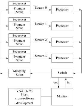
The prototype MUSE has four streams and associated with each of these is a Program Store and a Processor. The instructions have a five-field format with the first field containing the op-code, the next two the source operands and the last two the destination addresses of the result tokens (which could be sent to the same or to different streams). The Processor executes instruc-tions taken from the Program Store and any result tokens which are to be fed to other streams flow in a clockwise fashion around the pipelined ring architecture (see figure 1).
Store Program Sequencer
Stream 0
Processor
Store Program Sequencer
Stream 1
Processor
Store Program Sequencer
Stream 2
Processor
Store Program Sequencer
Stream 3
Processor
Matching
Store Switch
Monitor
out in
VAX 11/750 Host: cross-software
[image:4.594.151.426.80.436.2]development
Figure 1. A block diagram of the MUSE.
tokens during the course of executing the program. Although the instructions on any given stream are executed sequentially, with the aid of a conventional program counter, it is only possible to execute them if all of their operands are present. Thus, each instruction location in the Program Store has associated with it a corresponding ‘shadow’ location in the Matching Store which marks an instruction as being capable of execution if, and only if, all its operands are present.
The mechanisms for recognising whether an instruction is capable of execution when the program counter reaches it, are embodied in the Sequencer. This device transmits completed instructions to the associated Processor, which performs the required operation on the source operands and then sends any generated result tokens to the addresses specified in the destination fields.
2.2. Compiler Strategy
The compiler developed for MUSE accepts an input language of arithmetic expressions, assignment statement and conditionals expressed in a PASCAL-like notation. To illustrate the allocation of program code among the streams and environments we consider the arithmetic expression:
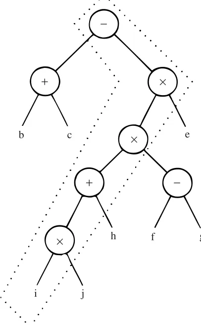
b+c−((i×j+h)×(f−g))×e
The successful evaluation of this expression requires, first of all, that each of the operands should possess a value. Moreover, in the tree diagram of figure 2, one can envisage, in classic data flow fashion, that the availability of operand values at the leaves of the tree causes the asso-ciated operators such as× and+ to function in parallel, and togenerate further values which are then passed higher up the tree.
Eventually the minus (−) operation at the root of the tree obtains two operands from its left and right branches and computes the final answer. It is clear that if all the branches of the tree contribute to the final answer, then the longest possible path from the root of the tree to a leaf operand will, in some sense, be the critical path in determining the overall speed of the calcula-tion. The critical path for the expression in question is shown within the dotted area of figure 2. It is an important part of the compiler strategy to identify this path and figure 3 shows how that path is mapped onto stream 0, environment 0 of the MUSE machine.
Other operands and sub-expressions are at first mapped onto the remaining streams in the same environment but when these streams are exhausted other environments are called into
+
+
×
×
×
−
−
b c e
g f
h
[image:5.594.201.404.370.698.2]j i
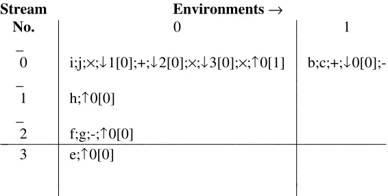
play. Thus, in figure 3 we note that the sub-expression (b+c) has been allocated to environment 1. Notation such as↓3[0] is read as “down three, zero” and means “await a result coming from stream three on environment zero”. Each such down (↓) operation is matched by a corresponding up (↑) operation. For example the down operation just mentioned is matched by the↑0[0] opera-tion on stream 3 which means “send the current result on this stream to the place on environment 0 and stream 0 where it is awaited by a down operation”. It will be clear that environment switch-ing takes place, to keep the stream processors busy, whenever a given environment becomes sus-pended on a ↓ operation which has not yet been activated by the receipt of a result from its matching↑ somewhere else in the machine. The encoding of the whole expression is in a postfix form with operands and operators separated by ‘;’ symbols.
Stream Environments→
No. 0 1
_
0 i;j;×;↓1[0];+;↓2[0];×;↓3[0];×;↑0[1] b;c;+;↓ 0[0];-_
1 h;↑0[0] _
2 f;g;-;↑0[0]
3 e;↑0[0]
[image:6.594.147.430.211.354.2]
Figure 3. Mapping program segments onto different environments.
Furthermore, if one starts at the top left of figure 3, writing down operands and operators as they are encountered but interpreting ↓ and ↑ arrows as directives to change stream and/or environ-ment, one obtains
ij x h + f g - x e x b c
+-which is, of course, the postfix form of the original expression. This makes it clear that the parti-tioning of the expression among the streams and environments corresponds to a ’flattening’ of the tree shown in figure 2.
Although the allocation strategy used by the compiler will, in most cases, distribute the computational load reasonably equitably between the available streams and environments, there are certain pathological cases where a particular tree shape, or the repetition of identical sub-expressions leads to a marked imbalance in the overall allocation. Some of these effects become apparent in the benchmarking tests described in later sections.
3. Modelling the Mk 0 MUSE.
Store Program Sequencer
Processor
Switch Matching
Store
Monitor
[image:7.594.144.433.77.335.2]out in
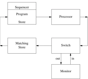
Figure 4. Initial Model for simulator.
The problem resolved itself into finding a suitable model for each of these constituent units. These models had to have the capacity to communicate with each other, via the interface units, in a well-defined manner, and to be functionally equivalent to their respective units. In addition, each sub-unit had to be totally asynchronous, and had to operate on a radically different time scale from every other.
In [6], simulation models are classified according to their types and features. A model is said to be “deterministic” if its action can be uniquely determined at any time, and “stochastic” if probabilistic factors must be considered. Further, a model can be “continuous” or “discrete” depending on the manner in which the data, parameters and relationships in the model change with time.
In the case of the MUSE, it was decided that a deterministic model was the most suitable in the first instance, because the primary use envisaged for the resulting program was in providing detailed timing information, and a stochastic model would imply that such timings could vary.
Furthermore, it was decided that the prototype could, in most cases, be thought of more nat-urally in the context of a discrete model, notwithstanding the fact that certain situations do have a continuous nature: for example when one component is waiting for a signal, and will begin action immediately upon its receipt. However, since all other events in the MUSE are driven by deter-ministic clocks providing predictable intervals, the advantages of this approach prompted a dis-crete approximation to the continuous cases. In a later section on approximations, this and other assumptions will be described in detail.
Accordingly the constituent units of the prototype MUSE were modelled as simple automata, and the interfaces between these parts were taken directly from the signals present in the prototype. To illustrate how this translation was accomplished, the modelling of the Processor module is explained in detail.
3.1. The Processor.
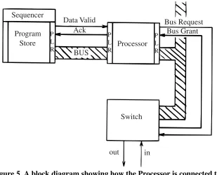
A Processor is required on each stream to execute instructions sent from the Program Store and to generate result tokens. The Processor is a microprogrammed bit-slice design and is described in detail in[3] but the following description briefly explains how the Processor executes instructions and how it interacts with its Program Store and the Switch. There is one Program Store and one Processor on each stream and each Program Store has an integral Sequencer sec-tion which is responsible for selecting the next instrucsec-tion to be executed. The 56 bit instrucsec-tions are sent one at a time from the Program Store to the Processor in accordance with the Sequencer protocol. The Processors generate 8-bit result values, tagged with their destination address, and these are then sent on to the Switch, where the destination address determines whether the results are sent to output devices or into the Matching Store.
3.1.1. Input and Output Interface.
Program Store Sequencer
Data Valid Ack
BUS
Processor
Bus Request Bus Grant
Switch
in out
P L R
P L R P
[image:8.594.135.444.314.564.2]L R
Figure 5. A block diagram showing how the Processor is connected to its Program Store and the Switch.
The interface between the Program Store and the Processor consists of a two-wire control link and a 56-bit data link and is shown in figure 5 where the pipeline register stages are repre-sented by “PLR”.
The Program Store issues a “Data Valid” signal when the next instruction has been selected by the Sequencer and it is available in the Program Store’s output register. The interface has a pipeline register and it allows the execution of the present instruction to proceed concurrently with the fetch of the next instruction. The “ack” signal is issued when the instruction has been loaded into the input register of the Processor.
to implement this. The arbitration logic is contained in the Switch.
When the Processor has completed the execution of its current instruction it loads the result value and destination address into its output register — as soon as this occurs the Processor may commence the execution of the next instruction. At this point the Processor also sends a “Bus Request” signal to the Switch and if none of the other processors requires the bus then the Switch will send a "Bus Grant" signal back to the processor causing it to output the information in its output register. The trailing edge of “Bus Grant” clears “Bus Request” and frees the output regis-ter for further generated results.
3.1.2. Operation of the Processor.
The microprogram tests the condition of the “Data Valid” signal received from the Program Store. The microprogram counter executes the same idling instruction until “Data Valid” becomes active, indicating that a new instruction is available from the Program Store. The new instruction is clocked into the input register of the Processor by the generation of an “Ack” signal by the microprogram. This signal also informs the Program Store that the instruction has been loaded into the Processor and that the Program Store may now commence assembling the next instruction.
The microprogram then issues a “JMAP” instruction. The opcode part of the instruction is used to address a mapping PROM which generates the required starting address of the operation routine in the microprogram. The required operation is performed on the two source operands (S1 and S2) and a result is generated. The actual duration of instruction execution is dependent on the operation performed e.g. add takes 1 micro-instruction, and multiply takes 12 micro-instructions.
When a result has been generated it is saved in one of the internal registers of the ALU and the microprogram then jumps to the output routine. If the first destination address, Dl, is a valid address then the result byte (stored in an ALU register) is loaded into the output register, pro-vided that register is empty. An internal Processor signal, “cbusy”, is used to indicate if the out-put register is full. When the result token is loaded into the register a "Bus Request" signal is gen-erated which informs the Switch that a bus access is required.
If D1 is the only valid output address then the Processor has completed the execution of the current instruction and the microprogram jumps back to the start and awaits a new instruction.
If the second destination address, D2, is also valid then a second output token must be gen-erated. It is possible at this point that the output register is still full and the microprogram would have to wait until the output register becomes empty again, which will be after the Switch accepts the previous result token. D2 is eventually loaded into the output register and the microprogram jumps back to the start.
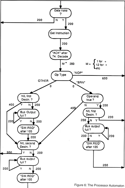
3.1.3. The Automaton.
To develop the automaton associated with the Processing unit, it was necessary to extract the atomic events for each of the steps specified above. This was achieved by taking each of the the microcode instructions and specifying automaton events for each. Because the microcode fol-lows clearly defined stages, the delays between the events could be determined and specified alongside the event transitions. Figure 6 shows the final automaton structure for this unit.
3.2. Implementing the Simulator.
The next few sections detail the decisions taken in writing the program, and show how a satisfactory strategy was eventually produced.
3.2.1. The Driving Mechanism.
We recall that it had been decided to use a discrete event model. Now, there are two obvi-ous methods for driving a discrete event simulation - by clock or by event [6]. In a clock-driven simulation — also known as “Fixed Time Step” mode — the simulator’s internal clock beats at a constant rate. For every tick, the events due to occur in that slot, if any, are performed. However, while being easy to arrange, this approach can be very wasteful in circumstances where long peri-ods of time may elapse between consecutive events.
By contrast, in an event-driven simulation, a list of “interesting” events is maintained. Each event has an associated time, by which the list is ordered, and the simulation progresses through the list executing the events in order until some “stop condition” — such as the end of the list — is met. As the events are executed, they may cause further events to be scheduled for some arbi-trary time in the future. The clock is always set equal to the time associated with the event due to occur, and so it becomes incremented by the appropriate amount rather than at a constant rate.
Now, because the finest increment of time in any of the automata is 1 ns, this was taken as the basic clock cycle, or “tick”. A Sequencer cycle is 50 ns and therefore 50 ticks, and a Proces-sor cycle is 200, but in practice an automaton state need not last for just one of that unit’s cycles. For instance, the decoding and execution state in the Processor automaton can take between two and thirteen cycles, depending on the operator type. This state can therefore last 2600 ticks in some cases. Clearly a clock-driven simulation, working on a 1 ns basic cycle, would be a mis-take; an event driven simulation was therefore chosen.
3.2.2. The Simulator Events.
The simulator events were derived from the state transitions in the various automata. For each of the constituent units, a procedure was written to perform the required action in any given state. Associated with each procedure was a “state variable”, by which the action was determined.
The procedures were written in such a way that each procedure call would result in a state transition for that particular automaton. That is, the desired action would be performed, the state variable modified to the new value, and another call of the procedure entered in the event list with the requisite delay into the future. When the next call of the procedure occurred, the state variable would again determine the appropriate action, and would be modified further. In this way, the automata were made to progress through their states in a controlled manner, maintaining the cor-rect delays.
In the prototype MUSE, there is only one instance of the Switch, Monitor and Matching Store, and so this approach was adequate for those sub-units. However, there are four streams, and hence four Sequencers and Processors, and it was hoped to simulate many more. To cope with this, a stream number was associated with each event in the event list, and passed as an argu-ment to the events as they were called. In the case of the Switch, Monitor and Matching Store this number could be ignored, but in the case of the Sequencer and Processor it was used to determine the stream concerned.
3.2.3. Simulating Concurrency.
An essential aspect of the MUSE design is the concurrent nature of each constituent unit. The Switch, Matching Store, Monitor, Sequencers and Processors may all act in a totally parallel and completely asynchronous manner and simulating such a system in an essentially sequential program was not always easy.
An early suggestion involved using distinct processes running under UNIX for each of the separate units, with a master program responsible for the shared data. The UNIX operating sys-tem primitives would have enabled process interactions to be controlled, and their operation could have progressed in as asynchronous a manner as is possible on a traditional time-shared computer system.
However, while having some definite advantages, this approach suffered from the inescapable problem of the upper limit to the number of processes per user, and one very impor-tant use for this simulator was to test the result of increasing the number of streams indefinitely. Clearly, this method would introduce an undesirable limiting factor, quite apart from the general slowing down of the simulator because of operating system overheads, and was rejected for these reasons.
Since a truly asynchronous simulation was impossible, it was decided that an approximation was necessary, and this was provided by the event list mechanism. Although the constituent units of the MUSE act concurrently within a macroscopic time frame, it is intuitively obvious that for a sufficiently small quantum of time the actions are sequential. It was decided that — to a first approximation — the 1 ns time-base used by the driving mechanism was indeed sufficiently small, and hence the events could be executed sequentially.
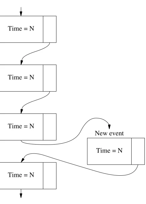
Now, the event list is ordered by time, with ‘simultaneous’ events being handled in the order in which they were entered. In the actual MUSE hardware, events at identical times would be executed simultaneously, but the simulator’s approximation means that these events are exe-cuted in the order in which they are found. Generally this is acceptable, but in certain circum-stances the Switch and Matching Store perform quite extensive actions within one tick. There-fore, to maintain the illusion of simultaneity, these actions are separated into states with instanta-neous transitions and to manage this, it became necessary to adopt the strategy of entering events into the event list at the end of a particular time “chain”. In this way a 1 ns time slot could be shared as required (see figure 7). Naturally, this overall approach raises certain problems, one major one being explained below. Nevertheless, it is felt to be the best method, and has the advantage of being easy to modify if new timings are required, or if new types of event are needed.
3.3. Assumptions and Approximations.
In producing the original model, and deriving a working and reasonably efficient program, a number of assumptions and approximations to the model were necessary. Several of these have been alluded to above; in this section these and others will be explained and justified.
3.3.1. The Initial Configuration.
Time = N
Time = N
Time = N
Time = N New event
[image:13.594.171.409.73.404.2]Time = N
Figure 7. Diagram of event list
The Switch automaton is responsible for providing each stream with a “window” of time, 100 ns long, in which it has unique access to the global bus. The initialisation routine produces a situa-tion in which stream 0 has access, and is at the start of its window at time 0.
Now, in the prototype MUSE, when the power is first turned on, the Switch begins cycling through the streams but only when activated do they commence execution. Clearly, the Sequencer and Processor actions in the hardware can begin anywhere within the Switch window, and with any stream number value. Thus, it is possible but unlikely, for the initial configuration of the simulator to match the configuration of the MUSE when activated.
3.3.2. Representing Continuous Events.
Although the simulation model of the MUSE was taken to be a deterministic, discrete event model, it is still the case, in the hardware prototype, that situations of a continuous nature may occur when one unit is waiting for a signal from another. Two such cases may arise between the Switch and the Monitor, and within the Sequencers.
In the former case, the Monitor is in an idle state initially, awaiting an interrupt from the Switch. This interrupt causes the Monitor to begin processing the output token, ultimately dis-playing it. At this time the Sequencer can be awaiting either the Processor’s “Acknowledge” sig-nal (indicating that the communicating pipline has been emptied), or the Matching Store’s “Re-quest” signal (indicating that new data is available).
was then responsible for detecting that the automaton was asleep and for arranging to “awaken” it. The signalling unit must be capable of determining whether or not the signalled unit is “active” by examining a shared flag, and of automatically making an entry in the event list for it if neces-sary. Clearly this requires the signalling unit to make use of information not present in the origi-nal model; in other words the units are bound together more closely in the simulation than in the original abstract automata or the hardware prototype. This extra hidden dependency made it nec-essary that great care be taken whenever the simulator was extended to investigate enhancements to the hardware.
3.3.3. The Occurrence of Events.
In the prototype, events occur over a given period of time. For instance, the Processor will require some 2600 ns to decode and execute a multiply instruction, and this action can be thought of as progressing in a continuous fashion whereas, in the simulation, this progression must be replaced by an occurrence of the event at a definite time.
The action of the Processor in the MUSE itself is divided into time intervals, each being a multiple of the Processor’s clock cycle of 200 ns. Within each of these intervals an action occurs — that is, before entry to the interval some condition may hold, and upon exit it does not but in general it is not possible to localise this action further within the interval.
In the simulation, on the other hand, the action is considered to occur instantaneously at the beginning of this interval, followed by a period of inaction. Hence the multiply instruction is sim-ulated by decoding and executing the instruction at a particular time, and then entering the next call of the Processor automaton, with a modified state variable, after 2600 ticks.
This approach, though adequate for program instructions, was not powerful enough for sig-nals. The interval during which a signal was to be generated by a particular component was known but a further period of time was necessary, for that signal to progress to another compo-nent and to become stable. This period could not be determined exactly, but an upper limit could be approximated. The signal was, therefore, considered to be generated within the particular interval, but actually set at the end of this period.
In order to manage these requirements in the program, the setting of a signal was made an event, with an associated procedure. The automaton concerned generated the signal by causing an occurrence of this event to be chained in the event list after the estimated period. This event, when executed, caused the signal to be set.
3.4. Validating the Simulator.
The simulator, model and prototype can be considered as a system. By careful construction and examination it is possible to be reasonably confident that the automata-based model is a valid representation of the hardware prototype, and that the simulator, is in turn, an accurate reflection of the model. However, only by comparison with the prototype can the simulator’s accuracy be proved.
To compare the simulator with the prototype, it was first necessary to find some parameter by which they could be calibrated with one another. The simplest of these was the time from the initiation of a given calculation to the output of the first token. The simulator program was altered to print the time at this point, and an accurate timing device was connected to the prototype machine.
The experiments were chosen with the intention of deriving representative timing informa-tion rather than data about the prototype’s performance in all possible situainforma-tions. With this in mind, the experiments were chosen so as to be simple and easily repeatable. Examples are the addition 1+2, on each of the environments in turn, and 120 additions of 1 to itself on increasing numbers of streams. Unfortunately, when the timings of these experiments on the prototype were compared with those of the simulator, a marked discrepancy was found.
It was possible for this discrepancy to have arisen from a fault in the model, or a mistransla-tion of this model in the program. In fact, a number of errors were located in both, the majority being minor clerical errors in the program but the model was also found to have a major fault in its representation of the Switch automaton.
The speed with which this automaton was corrected and replaced in the program was felt to be indicative of the ease with which wholly new architectures could be tested. Upon correction, the simulator produced consistently accurate timings (generally within 2% of the actual hardware values).
4. Evaluation of the existing Muse Architecture.
The Simulator described above was devised to allow a number of investigations of the MUSE structure to be carried out. These investigations were planned to explore the limitations of two very important features of the hardware design - the interconnection network which deter-mines the number of streams supported, and the sequencing mechanism, which deterdeter-mines the maximum number of environments available.
4.1. Communication Limitations.
In the first of these investigations, a general indication of the throughput of the MUSE structure was sought. The compiler strategy concentrates on distributing the assembly code over all the available streams as is available, and it was clearly important to know the maximum num-ber of streams which the time-multiplexed bus structure could adequately support.
Two factors were expected to influence the machine’s performance as more streams were added. More streams provide greater processing power and if the program can be distributed amongst the available streams it is possible for more instructions to be executed in parallel. Against this, however, is the problem of result communication. Instructions which are executed in parallel must transfer their result values in parallel. Consequently, the addition of more streams leads to greater bus contention and delays, as the Switch’s round-robin mechanism processes each request in turn. At some point these factors are balanced and no further improvements in execution speed will be observed as more streams are provided.
To assess these factors, a simple benchmark program was executed on a fixed number of streams, ranging from 1 to 16, and using potentially all 16 environments on each stream. This program produced 123 tokens and allowed 56 instructions to be executed concurrently if suffi-cient processing resources were available. The execution speed of the program is recorded in Graph 1. As expected, the graph rises up to a maximum, beyond which no further gain in perfor-mance is observed. The execution speed is seen to be around 1 MIPS at that point, and is reached at approximately 8 streams.
MIPS
Number of Streams 0
0.2 0.4 0.6 0.8 1 1.2 1.4
1 2 3 4 5 6 7 8 9 10 11 12 13 14 15 16
Graph 1: Small Benchmark on 16 Environments, 1–16 Streams. the results are shown in Graph 2.
MIPS
Number of Streams 0
0.2 0.4 0.6 0.8 1 1.2 1.4
1 2 3 4 5 6 7 8 9 10 11 12 13 14 15 16
Graph 2: Large benchmark on 16 Environments, 1–16 Streams.
Two important features are demonstrated in this graph. Unlike the smaller benchmark, the larger program possessed a high degree of regularity in its tree structure; each of 16 assignment operations being calculated by identically organised instructions. This resulted in large blocks of code being produced by the compiler which, in its stream allocation strategy, takes no notice of the size of the code blocks it assigns to particular environments. Accordingly it was possible for several of these large blocks of code to appear on a particular environment while its neighbouring streams or environments remained under-used.
A secondary feature of this graph, despite its many peaks and troughs, is that the same macroscopic performance pattern as already seen in Graph 1 re-emerges. A maximum execution speed of 1.3 MIPS is observed, reached at 9 Streams, which is in close agreement with the figure derived in the previous investigation.
From these preliminary investigations, it appears that the Mark 0 structure can only support up to 8 streams adequately, and that the maximum throughput of the system as a whole is of the order of 1 to 1.5 MIPS. Increasing this throughput would require that the interconnection network be improved and the speed of individual streams increased.
Clearly, the execution speeds of individual streams can be improved by constructing them from faster circuits, but there are physical limitations on this. Instead, it was decided to examine the potential for performance improvements which might result from changes in the environment switching mechanism.
4.2. Environmental Limitations.
The environment sequencing mechanism of the MUSE has been described in section 2.1. When new operand values arrive in the Program Store, the overhead for the Sequencer in finding them is directly proportional to the number of the environment block in which they are placed. We shall call this “proportional environment switching” and it occurs as a result of the way the prototype sequencer was designed.
To illustrate the effect of this mechanism, the smaller of the benchmark programs was allo-cated to a fixed number of environments, ranging from 1 to 32 in number and using 2 streams in every case. The reason why only 2 streams were used was to ensure that the effect of the global bus on the machine’s performance, from bus contention and token access collision, was at a mini-mum. The results of this investigation are shown in Graph 3.
MIPS
Environment Number 0
0.2 0.4 0.6 0.8 1
0 2 4 6 8 10 12 14 16 18 20 22 24 26 28 30 32
Graph 3: Benchmark on 2 Streams 1–32 Environments.
The execution speed of the program rises to a maximum of 0.7 MIPS at 3 and 5 environ-ments; it then drops steadily as more environments are added. The environment maximum of 16 imposed by the current hardware is seen on this graph to be barely superior to the case where only one environment was provided. This investigation implies that the environment sequencing mechanism is far from ideal, and that an environment maximum of 4 may be more realistic.
maximum execution speed is raised to 1 MIPS.
The environment sequencing mechanism is central to the concept of multi-stream evalua-tion; if the present mechanism can only support a maximum of 4 environments before the switch-ing overhead degrades performance, then clearly an improved system is required. A ‘non-proportional’ sequencing mechanism was therefore investigated with the aid of the Simulator.
On the existing prototype, when all the environments on any stream are unable to proceed, the Sequencer on that stream moves into an idle state and waits for an operand pair to be inserted in the Program Store. The Sequencer is alerted to the presence of new data, and
MIPS
Number of Streams 0
0.2 0.4 0.6 0.8 1 1.2 1.4
1 2 3 4 5 6 7 8 9 10 11 12 13 14 15 16
.... ....
... ....
.... .. . . .. . .. .
. . . .. .. . . .. . . .. . . .. . . .. . . .. . . .. . . .. . . ... . .. . . .... .. . ... .
Graph 4: Comparison of 16 (solid) & 4 (dotted) Environment usage.
hence of an enabled instruction, but it does not know the location of that instruction. Each of the environments must be examined, in turn, to find the instruction, and even then it is only exe-cutable if that instruction is pointed at by one of the appropriate program counters.
If the Sequencer could be informed of the environment in which the newly enabled instruc-tion was to be found then a non-proporinstruc-tional ‘vectored’ mechanism could be supported. Concep-tually this could be achieved by associating a flag with each of the environments, which, when set, would indicate that the environment could be executed - that is, the instruction referenced by the environment program counter had become enabled. The initial values for the flags could be set by the downloading software and then maintained by the Sequencer as the code was executed. In addition, the Matching Store would need to set the appropriate environment flag whenever it inserted new operand data but the Sequencer would only need to examine the current instruction on that environment To allow the Matching Store to know which environment flag to set, an envi-ronment destination field, in addition to the stream and instruction number fields, would be neces-sary.
Rather than altering the assembler, downloader and simulator to support this additional des-tination field, it was realised that the effect of such an alteration could be mimicked in the simula-tor. by simply removing the delays in the Sequencer’s environment search loop.
MIPS
Number of Streams 0
0.2 0.4 0.6 0.8 1
0 2 4 6 8 10 12 14 16 18 20 22 24 26 28 30 32
....
.... . ... . . .. . . .. . . .. . . .. . . .. . . ... . .. .. . . .. . . .. . . .. . . .. . . .. . . .. . . .. . . .
Graph 5: Comparison of proportional (solid) & non-proportional (dotted) mechanisms.
This investigation indicates that non-proportional environment sequencing allows a greater number of environments to be supported than the original system. Graph 6 illustrates the effect that this has on the 1 to 16 Stream range when 16 environments are used; the machine’s perfor-mance is improved over the whole stream range and the maximum execution speed is raised from 1 to 1.1 MIPS. In terms of performance improvement this is not particularly impressive, but Graph 5 shows that the environment maximum can be at least doubled by employing this new mechanism.
5. Discussion.
The experiments described in the previous section highlight the limitations imposed by the communication network and by the Sequencer design. Architectural improvements for these par-ticular features are described below, together with some more general suggestions for
MIPS
Number of Streams 0
0.2 0.4 0.6 0.8 1 1.2 1.4
1 2 3 4 5 6 7 8 9 10 11 12 13 14 15 16
. .. . . .. .
... ....
.... ... . . .. . .. . .
. . .. .. . . .
.. . . .. . . .. . . .. . . .. . . .. . . .. . . .. . . .. . . .. . . .
5.1. Communication
The relative timings between the Processors and the Switch, described in section 3.1.1, are shown in more detail, in figure 8, for one particular stream. In the ensuing discussion we assume that this is stream number 2.
Bus Request 2
Bus Grant 2
Figure 8. Processor and Switch interface timing.
During the period fromt1 tot2 it is assumed that one of the other streams is using the bus and stream 2 has to wait until the other stream has completed the transfer. During the period from t2 to t3 stream 2 is granted access and the result token is placed on the bus. It can be seen that there may be a long delay before the Processor can transfer its result and this may be due to either another stream using the bus or due to the round-robin rotating priority mechanism.
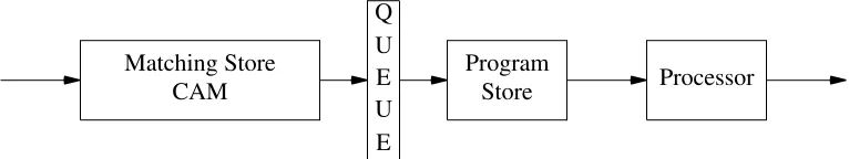
This type of communication system is clearly unsuitable for interconnecting large numbers of processors and would scarcely cope with more than the four streams in the prototype. One con-tribution towards reducing the traffic on the bus would be to eliminate the need for explicit DUP (Le. ’duplicate’) instructions, which have to be generated whenever a result is required at several destinations. A form of Content Addressable Memory is currently being evaluated which only requires one input, but may produce many outputs depending on where the result is required. A conceptual view of this is shown below in figure 9 and it can be seen that the global Matching Store has been split and moved onto the Stream itself. Placing the Matching Store on the streams in this way would also allow a local communication path to be utilised for transferring results that are needed on the same stream or environment that is currently in use.
Matching Store CAM
Q U E U E
Program
[image:20.594.97.480.443.515.2]Store Processor
Figure 9. Using CAM to reduce token communication overheads.
The FIFO (first-in, first-out) queue is used to store the (possibly many) operands that may be produced by the CAM.
Other methods for interconnecting the streams are under investigation; one possibility being the use of crosspoint switches as in the March Hare network switching device[9].
5.2. Sequencer Problem
5.3. General
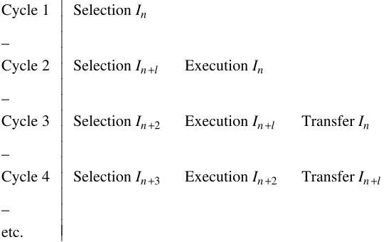
In the prototype MUSE each stream is split into three pipeline stages. These are shown in figure 10 and consist of instruction selection by the Sequencer, instruction execution by the Pro-cessor and the storage of the result prior to transfer by the Switch. This pipelining allows concur-rent activity to take place and figure 11 shows how the selection of the next instruction is carried out during the execution of the first instruction. (As in all pipeline designs there is an initial period during which the pipeline is being filled.)
Selection
P L R
Processor
P L R
Switch
[image:21.594.74.504.181.284.2]P L R
Figure 10. The Pipeline Stages in the MUSE.
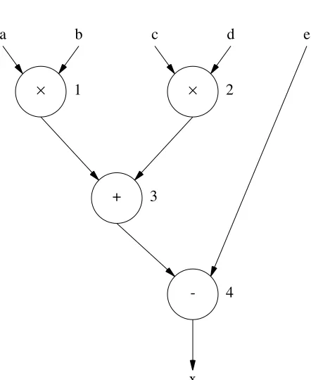
In most parallel processing architectures pipelining is an asset but in MUSE its use may have a detrimental effect. Unstructured data-driven computers rely on the fact that instructions may be executed as soon as their operands are available and the presence of data is their sole cri-terion for possible execution. In the MUSE, instruction execution is related to the execution of other instructions and we require these sequences of instructions to be executed as efficiently as possible, but, by using pipeline stages there may be a delay in obtaining the result of a calcula-tion. To make this point clearer figure 12 shows part of a program tree to calculate the subexpres-sion (a×b)+(c×d)−ein which the instructions labelled 1, 3 and 4 would probably be
Cycle 1 SelectionIn
_
Cycle 2 SelectionIn+l ExecutionIn
_
Cycle 3 SelectionIn+2 ExecutionIn+l TransferIn
_
Cycle 4 SelectionIn+3 ExecutionIn+2 TransferIn+l
_
etc.
Figure 11. Selection, execution and transfer of the instructions.
[image:21.594.71.346.447.617.2]a b c d e
× ×
+
-x
1 2
3
[image:22.594.178.399.77.347.2]4
Figure 12. A program tree of the sub expression (a×b)+(c×d)−e
Cycle 1 Selection Inst. 1
_
Cycle 2 Execution Inst. 1
_
Cycle 3 Transfer Inst. 1
_
Cycle 4 Selection Inst. 3
_
Cycle 5 Execution Inst. 3
etc.
Figure 13. Instruction selection and execution for the program tree of figure 12.
The environment switching mechanism will alleviate this problem to a certain extent in that other instructions may be selected and executed during cycles 2 and 3 but if instructions 1,3 and 4 do indeed form a critical path (or a working set in the terminology of Tokoro et. al.[10]) then the overall execution of the program will be slowed down. The more pipeline stages there are the worse the problem becomes.
[image:22.594.75.378.401.600.2]further pipeline stages (figure 14). Notice that the global Matching Store of the prototype needs to be split up and distributed over all of the streams in order for the idea of a local communication path to be efficiently realised.
Matching Store
Program Store Sequencer
P L R
[image:23.594.101.475.136.221.2]Processor Result token
Figure 14. Using a Local Communication Path. 6. Conclusion
One outcome of these investigations has been to confirm, very emphatically, the value of a properly calibrated software simulator for investigating novel computer architecture. All of the perceived advantages of this approach, as listed in section 1, were amply confirmed in practice. But, as with any simulation, it would have been quite impossible to be confident in any of its pre-dictions if it had not been carefully compared with the actual performance of the hardware proto-type over the ranges of stream and environment numbers where such a comparison could be made. It was a truly sobering experience to find, time and time again, how some gross mismatch in performance as predicted by the hardware prototype and the software simulation, was traced to the existence of some deep-seated problem in the simulator. On the other hand, it was reassuring to find that whenever architectural improvements suggested by the simulator were capable of being implemented on the original hardware the timings agreed to within a few per cent.
A second major insight has been to appreciate how the enormously increased communica-tion requirements of fine-grain parallelism can quickly swamp any communicacommunica-tions system and thereby negate any increase in speed that might have occured from the exploitation of the inher-ent parallelism of the problem. We consider it vital that potinher-ential ‘critical paths’ and local ‘work-ing sets’ be identified as our compiler attempts to do. Moreover, it is clear that some local high bandwidth communication path has to be provided for such ‘local’ results, leaving the global communication mechanism for transmitting results to portions of the program that truly are more remote e.g. calls of procedures.
Acknowledgements
We thank the other members of the MUSE project team for their support and continued enthusiasm for the project.
The construction of the hardware was financed by Plessey Office Systems, Beeston, Not-tingham to whom we are also grateful, in conjunction with the Science and Engineering Research Council of Great Britain, for the provision of a CASE studentship for James Duckworth.
References
1. R.J. Duckworth,Parallel Computation on a Multi-Stream Data Flow Machine, University of Nottingham, October 1984. PhD. Thesis
3. R.J. Duckworth, D.F. Brailsford, and L. Harrison, "A Structured Data Flow Computer," Proceedings of the IlEE, vol. Pt. E. Submitted Oct 1985
4. J. R. Gurd, C. C. Kirkham, and I. Watson, “The Manchester Prototype Dataflow Computer,” Communications of the ACM, vol. 28, no. 1, pp. 34–52, January 1985.
5. N.K. Barrett, Software Tools and a Simulation System for the Nottingham Multi-Stream Dataflow Project, University of Nottingham, 1985. Ph.D. Thesis
6. Samuel L. S. Jacoby and Janusz S. Kowalik, Mathematical Modelling with Computers, Prentice-Hall International, 1980.
7. James L. Peterson,Petri Net Theory and the Modelling of Systems, Prentice-Hall Interna-tional, 1981.
8. John E. Hopcroft and Jeffrey D. Ullman,Introduction to Automata Theory, Languages and Computation, Addison-Wesley, 1979.
9. M.D. Cripps and A.J. Field,The MARCH HARE Network Switching Device, Imperial Col-lege of Science and Technology, March 1983. Research Report DOC 83/30, Department of Computing.