Numerical Calculation of Geoelectric Fields That Affect Critical Infrastructure

(1)

https://www.scirp.org/journal/ijg ISSN Online: 2156-8367

ISSN Print: 2156-8359

DOI: 10.4236/ijg.2019.1010053 Oct. 29, 2019 930 International Journal of Geosciences

Numerical Calculation of Geoelectric Fields

That Affect Critical Infrastructure

David H. Boteler, Risto J. Pirjola

Geomagnetic Laboratory, Natural Resources Canada, Ottawa, Canada

Abstract

One of the modern applications of geomagnetism is determining the effect of geomagnetic disturbances on critical infrastructure such as power systems and pipelines. Assessing the geomagnetic hazard to such systems requires calculation of the geoelectric fields produced during geomagnetic distur-bances. Such geoelectric fields can then be used as input to system models to calculate the impact on the system. This paper describes what is involved in calculating the geoelectric fields produced during real geomagnetic distur-bances. The theory of geomagnetic induction is presented and used to derive the Earth transfer function relating the geoelectric and geomagnetic field var-iations at the Earth’s surface. It is then shown how this can be used to make practical calculations of the geoelectric fields and how the calculation process can be verified by comparison with analytic solutions obtained with synthetic geomagnetic variation data. The accuracy of the calculated geoelectric fields for geomagnetic risk assessments is limited, not by the accuracy of the calcu-lation methods, but by the availability of geomagnetic field measurements and Earth conductivity information over the whole extent of the affected in-frastructure.

Keywords

Geoelectric Fields, Geomagnetic Disturbances, Critical Infrastructure, Hazard Assessment

1. Introduction

Geomagnetism has always been an applied science because of the use of the magnetic field for navigation purposes, e.g. [1][2]. In modern times a new ap-plication of geomagnetism has arisen. This follows the recognition that technol-ogical systems using long conductors can be affected by the geomagnetically

in-How to cite this paper: Boteler, D.H. and Pirjola, R.J. (2019) Numerical Calculation of Geoelectric Fields That Affect Critical In-frastructure. International Journal of Geos-ciences, 10, 930-949.

https://doi.org/10.4236/ijg.2019.1010053

Received: September 21, 2019 Accepted: October 26, 2019 Published: October 29, 2019

(2)

DOI: 10.4236/ijg.2019.1010053 931 International Journal of Geosciences

duced currents (GIC) produced during geomagnetic disturbances [3]. The tele-graph was the first system to suffer from natural voltages [4], and in 1859 the “Carrington storm” caused disruption to telegraph systems around the world [5]. Pipelines represent another type of long conductor subjected to geomagnetic induction. In this case, geomagnetic induction gives rise to “telluric currents” in the pipeline that may enhance corrosion and interfere with the corrosion pre-vention systems for the pipeline [6] [7]. Starting in 1940, geomagnetically in-duced currents proin-duced in high-voltage power transmission systems during large geomagnetic disturbances have led to equipment damage and power black-outs [8][9][10][11]. Concern about these effects has led to extensive work to understand the geomagnetic effects and to assess the hazard they pose to the op-eration of these systems, e.g. [12][13][14].

Assessing the geomagnetic hazard to grounded networks requires the use of geomagnetic field data and Earth conductivity models to calculate the geoelectric fields experienced by the system. The calculated geoelectric fields can then be used as input to system models to evaluate the geomagnetically induced currents (telluric currents) and the associated voltages and their impacts on the system. The method presented here uses standard theory widely used before, e.g. [8][15] [16][17]; however, the details of the numerical calculations are usually ignored and can lead to errors if not done correctly.

The purpose of this paper is to present the numerical method for calculation of the geoelectric field. However, to show the origin of the relations used, we first present the theory of geomagnetic induction starting from Maxwell’s equa-tions and show how this is used to derive the Earth transfer function relating the geoelectric field to the geomagnetic field variation at the Earth’s surface. Then we show how these calculations can be made in practice using a time series of sampled geomagnetic field data. Further, we show how the numerical calculation can be tested by use of synthetic magnetic field data and comparison of the cal-culated geoelectric fields with analytic solutions obtained for two test cases. Fi-nally, the source of the Earth conductivity models is described and we discuss how limitations in the availability of such information influence the accuracy of geomagnetic hazard assessments.

2. Theory

The relations between electric and magnetic fields at the Earth’s surface are go-verned by Maxwell’s equations. For geomagnetic induction in the Earth we are dealing with frequencies ƒ and conductivities σ such that σ 2πfε0 where ε0

= 8.854 × 10−12_{F/m is the permittivity of free space. Consequently, the} displace-ment current term associated with 2πƒε0 is negligible and can be dropped from Maxwell’s equations. Thus the equations can be written as

t

∂ ∇× = −

∂ B

E (1)

0

µ σ

(3)

where bold denotes vectors and μ0 = 4π × 10−7 H/m is the permeability of free space assumed to be valid in the Earth, too. Any geoelectric field E(t) and geo-magnetic field variation B(t) can be expressed as the sum (i.e. an inverse Fourier transform) of their frequency components, ƒ:

( )

2

ei ftd

t f f

∞

π

−∞ =

_∫

E E (3)

( )

2

ei ftd

t f f

∞

π

−∞ =

_∫

B B (4)

where i= −1.

The rate of change of the magnetic field denoted by g(t) can then be written as

( )

d

( )

2

2 e d

d

i ft

t

t i f f f

t

∞

π

−∞

= B =

_∫

π

g B (5)

Substituting (3), (4) and (5) into (1) and (2) then gives equations

( )

2

( )

2

ei ftd 2 ei ftd

f f i f f f

∞ ∞

π π

−∞ −∞

∇×

_∫

E = −

_∫

πB (6)

( )

2

( )

2

0

ei ftd ei ftd

f f µ σ f f

∞ ∞

π π

−∞ −∞

∇×

_∫

B =

_∫

E (7)

Equations (6) and (7) imply that, in the frequency domain, E(ƒ) and B(ƒ) satisfy the following equations

( )

f i2 f

( )

f

∇ ×E = − πB (8)

( )

f µ σ0

( )

f

∇ ×B = E (9)

Using the standard geomagnetic xyz coordinate system in which the Earth’s surface is the xy plane and x, y and z refer to the northward, eastward and verti-cally downward directions, respectively, Equation (8) can be written in compo-nent form as follows

(

)

2

y x y x

z z

x y z

E E E E

E E

i f B B B

y z z x x y

∂ ∂

∂ ₋  ₊∂ ₋∂  ₊ ₋∂  _{= − π} ₊ ₊

 _∂ _∂  _ _∂ _∂ _  _∂ _∂ 

 i j  k i j k (10)

where i, j and k are the unit vectors in the x, y and z directions, respectively. For clarity, the dependence of the electric and magnetic components on the fre-quency ƒ is not explicitly shown in Equation (10). A common assumption made is that the horizontal spatial variations of the fields are much less than the varia-tion with depth (i.e. the skin depth in the Earth is much smaller than the hori-zontal spatial scales of the fields). This assumption is generally valid when “large-scale” ionospheric-magnetospheric sources are considered or the points of observation are far from the sources, and there are no significant lateral varia-tions in the Earth’s conductivity. In this case, the terms with the variation in the vertical direction (z) dominate on the left-hand side of Equation (10), and so Equation (10) reduces to

(

)

2

y x

x y z

E E

i f B B B

z z

∂ ∂

− + = − π + +

(4)

Equating the i, j and k components on both sides of Equation (11) gives

2

y

x E

i fB

z

∂

= π

∂ (12)

2 x

y

E

i fB

z

∂ _{= − π}

∂ (13)

and Bz = 0.

Thus a “transfer function” K = K(ƒ) can be defined that relates the orthogon-al electric E = E(ƒ) and magnetic B = B(ƒ) field components in the frequency domain at the Earth’s surface, i.e.

( )

( ) ( )

E f =K f B f (14)

where E(ƒ) and B(ƒ) can represent the relation between either Ex(ƒ) and By(ƒ) or −Ey(ƒ) and Bx(ƒ) .

This transfer function K(ƒ) is closely related to the “surface impedance”

Z(ƒ) commonly used in geoelectromagnetic studies: Z(ƒ) = μ0K(ƒ) . The elec-tric field can also be related to the rate of change of the magnetic field, g(t) =

dB(t)/dt. Noting that in the frequency domain g(ƒ) = i2πƒB(ƒ) (see Equation (5)) we obtain from (14)

( )

( ) ( )

( )

2

( )

( ) ( )

2

K f

E f K f B f i fB f C f g f

i f

= = π =

π (15)

where C(ƒ) given by

( )

2

K f C f

i f

=

π (16)

is called the “magnetotelluric relation”. It should also be noted that C(ƒ) is equal to the complex skin depth p(ƒ) often used in geoelectromagnetic investigations.

To determine the transfer function, K(ƒ) , take the curl of Equation (8). Using Equation (9) and noting that ∇ ⋅E

( )

f =0, we then obtain at each frequency

( )

2 2

f k f

∇ E = E (17)

where the propagation constant k = k(ƒ) is defined by

( )

2 0

k=k f = i πf

µ σ

(18)

Expanding (17) gives

2 2 2

2

2 2 2 k

x y z

∂ ∂ ∂

+ + =

∂ ∂ ∂

E E E

E (19)

Assuming again that the terms involving the variation with z dominate, Equa-tion (19) reduces to

2 2

2 k

z

∂ = ∂

E

E (20)

(5)

first if the Earth is approximated by a uniform conductivity model, and the second if the Earth is approximated by a layered conductivity model. The second option provides a model that represents the change of conductivity with depth in the Earth. Taking account of lateral changes in conductivity is briefly considered in Section 6.

2.1. Uniform Conductivity Model

A simple first approximation is to model the Earth by a half-space of uniform conductivity σ. In this case, Equation (20) has a solution of the form

( )

0 e

k f z

f = f −

E E (21)

where E0(ƒ) is the (vector) amplitude of the electric field at the Earth’s surface,

i.e. at z = 0, and k(ƒ) is given by Equation (18). Substituting the x or y compo-nents of E(ƒ) given by (21) into Equations (12) and (13) gives

2 y

x

E i f

B k

−

= π ₍₂₂₎

2 x

y

E i f

B = k

π

(23)

Equations (22) and (23) show that each pair of electric and magnetic field components form an orthogonal right-handed pair where the electric field is ro-tated 90 degrees counter clockwise from the direction of the magnetic field and the transfer function, K(ƒ) represents the relationship between Ex and By and between −Ey and Bx. These equations, utilizing (18), show that in the uniform-Earth case K(ƒ) is given by

( )

0

2 2

i f i f

K K f

k = µ σ

π π

= = ₍₂₄₎

2.2. Layered Conductivity Model

In practice the Earth conductivity varies in all directions, but the greatest varia-tion is with depth and the Earth is often represented by a one-dimensional (1-D) model comprised of N horizontal layers with specified conductivities (σ1,,σN)

and thicknesses (l1,,lN). Note that the bottom layer is a uniform half-space,

so lN = ∞.

As above, we assume that the horizontal variations of the electric and mag-netic fields are much less than the variations with depth, i.e. the fields are consi-dered to only depend on the z coordinate. Then the electric field satisfies Equa-tion (20) in each layer with kn= i2πf

µ σ

0 n (n=1,,N). As in Section 2.1,

we consider an (E, B) pair where E and B denote either Ex and By or −Ey and Bx. In the layered-Earth case the solution of Equation (20) needs to allow for up-going waves resulting from reflections at layer boundaries (not present in the uniform-Earth case). Then the solution for E from (20) is

ek zn ek zn

n n

(6)

where 0 ≤ z ≤ ln and Sn and Rn are the amplitudes of a downward and an upward propagating wave at the top surface of layer n, respectively (note that, for each layer, the location of z = 0 is set at the top surface of the particular layer, not at the Earth’s surface). The bottom layer N is a uniform half-space, so RN = 0.

Substituting E given by (25) into (12) or (13) yields

(

e e

)

2

n n

k z k z

n

n n

k

B S R

i f

−

= −

π (26)

As defined by Equation (14), the transfer function K = K(ƒ) relates E and B at the Earth’s surface. Let us denote the ratio of E to B at the top surface of layer n

by Kn. The bottom layer (i.e.n = N) is a uniform half-space so the value of KN is directly obtained from Formula (24) with σ = σN. Thus

0

2 2

N

N N

i f i f

K

k µ σ

= π = π (27)

For each layer above, Equations (25) and (26) are combined and we set z=0

togive the ratio of the fields at the top of the layer, i.e.Kn, and set z=l to give the ratio of the fields at the bottom of the layer which, because of continuity of fields across the boundary, is the same as the ratio of the fields at the top of the underlying layer, i.e. Kn+1,

n n n n n n S R K S R η + =

− (28)

1

e e

n n n n

k l k l

n n

n n k l k l

n n S R K S R η − + − + =

− (29)

where n 2 n

i f

k

η = π _{is the “}_{Characteristic Function}_{” of layer}_n_.

Dividing the top and bottom of Equation (29) by ek ln n gives

2 1 2 e e n n n n k l n n

n n k l

n n S R K S R η − + − + =

− (30)

Multiplying by the denominator on the right-hand side gives

(

2

)

(

2

)

1 e e

n n n n

k l k l

n n n n n n

K + S − −R =η S − +R (31)

Collecting terms in Sn and Rn gives

(

)

2

(

)

1 e 1

n n

k l

n n n n n n

K ₊ −

η

S − = K ₊ +

η

R (32)

Thus we can write

(

)

(

11

)

2

e n n

n n k l

n n n n K S R K η η + − + − =

+ (33)

Using this expression for Rn we can write

(

)

(

11

)

(

11

)

2

e n n

n n n n k l

n n n n

K K

S R S S

K K η η η η + + − + + + − + = +

+ + (34)

(7)

(

)

(

11

)

(

11

)

2

e n n

n n n n k l

n n n n

K K

S R S S

K K η η η η + + − + + + − − = −

+ + (35)

Substituting these into Equation (28) and cancelling common terms give

(

) (

)

(

) (

)

2 1 1 2 1 1 e e n n n n k l

n n n n

n n k l

n n n n

K K K K K η η η η η − + + − + + + + − =

+ − − (36)

Collecting terms in Kn+1 and ηn gives

(

) (

)

(

) (

)

2 2 1 2 2 1

1 e 1 e

n n n n

k l k l

n n

n n _{k l} _{k l}

n n K K K η η η − − + − − + + + − =

− + + (37)

Formula (37) is a recursive relation for calculating Kn at the top surface of layer n from Kn+1 at the top surface of the underlying layer n + 1. The initial

value in the application of Formula (37) is KNgiven by Equation (27) which is used to calculate Kn at the top surface of the next layer up. This is then used in the calculation for the next layer, and so on, up to the Earth’s surface. The final value is the transfer function K = K1 relating E and B at the Earth’s surface.

It should be noted that the multi-layer transfer function is exact, as is the uni-form-Earth transfer function, but in the multi-layer case the transfer function can only be expressed by the recursive relation (37) with the initial value from (27) whereas the transfer function for a uniform Earth has a simple explicit Formula (24).

The calculations are repeated for each frequency required to build up the full description of the dependence of the transfer function on frequency.

2.3. Expression for the Geoelectric Field

To determine the time variation of the electric field, we use Equation (3) and note that each frequency component of the electric field is given by the transfer function and the magnetic field at that frequency (Equation (14)). Thus we ob-tain

( )

( ) ( )

2

ei ftd

E t K f B f f

∞

π

−∞

=

_∫

₍₃₈₎

As shown in Sections 2.1 and 2.2, the Earth transfer function, K(ƒ) , can be derived as a function of frequency for a uniform conductivity model or a layered conductivity model of the Earth. To use this to calculate the geoelectric field, note that the B(ƒ) terms in (38) are given by the Fourier transform of the geo-magnetic field variation B(t). Thus (38) can be written as

( )

2 2

ei ftd ei ftd

K f B t t f

E t

∞ ∞

′

− π π

−∞ −∞   ′ ′    = 

∫

(39)

This can be more simply written

( )

1

( )

{

( )

}

E t =F− _K f F B t _ (40)

(8)

Thus the calculation of the geoelectric field comprises three steps: 1) Take the Fourier transform of the geomagnetic field variation B(t):

2) Multiply each frequency component by the transfer function of the Earth

K(ƒ) :

3) Take the inverse Fourier transform to obtain the geoelectric field E(t).

3. Sources of Data

Equation (39) shows that the calculation of geoelectric fields requires a time se-ries of magnetic field measurements B(t) and the Earth transfer function K(ƒ) dependent on the Earth’s conductivity structure.

3.1. Magnetic Field Measurements

Measurements of the Earth’s magnetic field are made at many observatories around the world. Most observatories are members of Intermagnet, which pro-motes common instrument standards and data collection methods. Data from Intermagnet observatories are available through the Web site

http://www.intermagnet.org. In addition, a number of magnetometer chains are operated by universities and research institutes, and these data have been col-lected together on the web site http://supermag.jhuapl.edu/mag/.

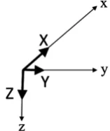
Magnetic field measurements are typically made using Fluxgate magnetome-ters. A set of three orthogonal magnetometers are used to measure the X, Y and

Z magnetic field components in the northward, eastward and vertically down-ward directions, respectively (Figure 1).

Magnetic field recordings have traditionally been made with a sampling in-terval of one minute, with higher frequencies filtered out prior to sampling to remove frequencies above the Nyquist frequency to prevent aliasing problems [18]. Recordings have also been made with sampling once every 10 s, or once every 5 s, and the new Intermagnet standard for observatories is to make re-cordings with a sampling interval of 1 s.

3.2. Earth Transfer Function

[image:8.595.332.411.600.694.2]

The Magnetotelluric (MT) technique is a geophysical method that uses record-ings of the geoelectric field and geomagnetic field variations to obtain informa-tion about the Earth conductivity structure [19][20][21]. Because the fields at

(9)

different frequencies penetrate to different depths within the Earth, spectral analy-sis of the geoelectric and geomagnetic field recordings can be used to determine the relationships between E and B at different frequencies and build up a (1-D) profile of the Earth conductivity variation with depth. Magnetotelluric surveys along transects or in arrays can be used to provide 2-D or 3-D models of the Earth conductivity structure.

The results from MT studies can be used in several ways. Published results from MT surveys usually describe the conductivity structure. These can be used to construct a 1-D layered Earth model, which is then used to calculate the Earth transfer function as shown in Sections 2.1 and 2.2. The MT results may show different conductivity values in different zones and a 1-D model can be con-structed for each zone with the results being used to obtain “piecewise” calcula-tions of the geoelectric fields affecting critical infrastructure [22]. Alternatively, where they are available, 2-D or 3-D models could be used to determine the transfer functions at the Earth’s surface.

Magnetotelluric studies, in the course of their data processing, generate sur-face impedance functions for each of their measuring sites. Some studies make these impedance functions available online (e.g. the Lithoprobe studies in Cana-da available at http://lithoprobe.eos.ubc.ca/and the Earthscope studies in the US available at http://www.earthscope.org. Using the relation K(ƒ) = Z(ƒ)/μ0, the sur-face impedance Z(ƒ) directly gives the Earth transfer function K(ƒ) to be ap-plied to the calculation of the geoelectric field.

4. Numerical Calculations

The first main step in numerical calculation of geoelectric fields, as specified in Section 2.3, is to take the Fourier transform of the magnetic field data for the in-terval of interest. However, before taking the Fourier transform some precondi-tioning of the magnetic field data is needed. This follows standard practice for time series analysis, e.g. [18]. To reduce spectral leakage it is desirable to remove the mean and linear trend from the time series and taper the ends by multiplying the time series with a split cosine bell window (or another suitable window). The split cosine bell window is given by

( )

(

)

1 2

1 cos , 0

2 2

1, 1

2 2

2 1

1

1 cos , 1 1

2 2

p

t p

p p

w t t

t p

   

− ≤ <

   

 

  



= ≤ < −



   − 

 _ −  _ − ≤ <

   



π

(41)

(10)

rec-DOI: 10.4236/ijg.2019.1010053 939 International Journal of Geosciences

ommended that the days on either side be included in the time series for analy-sis. The geoelectric field is then calculated for the set of 3 days and the results for the first and last day, which are affected by the tapering, are discarded leaving the correct geoelectric field values for the middle day of the set.

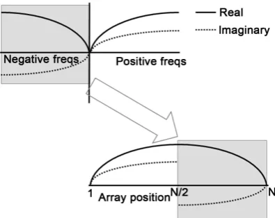
The Fourier transform of the geomagnetic data time series can be performed using a Fast Fourier Transform (FFT) that is built into many software packages. There is no standard convention for the definition of a forward transform or an inverse transform and these can differ from one software package to another. Fortunately, in this application where the forward and inverse transforms are always used as a pair, the choice of definition does not matter, although this is not the case when an individual transform is used [24]. Many FFT routines ex-pect the input data to be of a length that is a power of 2 and be comprised of complex numbers. This is easily achieved by padding the geomagnetic data set with zero values at the end to extend the data length to a power of 2 and by as-signing the geomagnetic data values to be the real parts and setting the imagi-nary parts to zero. This complex array is often overwritten by the output array from the FFT routine.

The Discrete Fourier Transforms to go between the samples of the continuous time recording (x) and discrete frequency components (X) can be defined as [24] [25].

( )

1

( )

2

0

1

e kn

N _i

N

n

X k x n

N

π

− ₋

=

∑

₍₄₂₎

( )

1

( )

2

0

e kn

N _i

N

n

x n X k

π −

=

∑

₍₄₃₎

[image:10.595.274.472.548.705.2]

When performing the forward FFT from the time domain to the frequency domain the output is the complex spectral components at positive and negative frequencies. However, the negative frequency components are output at the end of the array (Figure 2), which is a mathematical property of the Discrete Fourier Transform, not just a property of the FFT routine used. This needs to be taken into account when multiplying by the Earth transfer function values.

(11)

The output of the FFT is the spectral components of the magnetic field varia-tion at a set of frequencies determined by the time-domain sampling interval, ∆t, and the length of the time series, N, in the time domain that is transformed. These frequencies

1 1

1 2 2 ₂ 2 2 1

0, , , , , , , , ,

i

N _N N

f

N t N t N t N t N t N t N t

   

+_ − _ ₊ −_ − _

+ + _ _ _ _ − −

=

∆ ∆  ∆ ∆ ∆  ∆ ∆ (44)

are those for which the Earth transfer function must be calculated. For each of the positive frequencies multiply the magnetic field spectral value by the Earth transfer function to give the corresponding electric field spectral value. The elec-tric field spectral values for negative frequencies should then be set to the com-plex conjugates of the values for positive frequencies.

The resulting electric field spectrum (as with the magnetic field spectrum) has an even real part and an odd imaginary part. The odd imaginary part goes through zero at the Nyquist frequency (ƒN = 1/2∆t) (and at zero frequency). This requires setting the imaginary part of the E spectrum at ƒN equal to zero.

Now perform an inverse FFT on the electric field spectrum. This will give an array of complex values that contains the electric field in the time domain. Just as with the original magnetic field data, the electric field data must be real. Thus the computed array of electric field values should comprise complex values for which the imaginary parts are all zero. In practice, non-zero values are obtained for the imaginary parts but these should be many orders of magnitude (~10) smaller than the real part values. This should be checked as a test that the calcu-lations have been made correctly. Small differences in the above procedure, e.g. not setting the imaginary part at ƒN to zero can make the imaginary parts of the computed electric field values much larger than they should be.

5. Verification of the Calculations

Analytic expressions have been derived for synthetic magnetic test data and electric fields at the surface of a uniform Earth and a layered Earth [26][27].

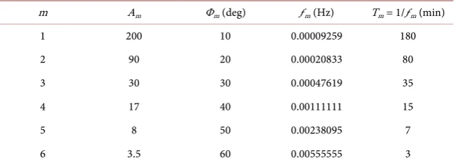
A synthetic test magnetic field variation has been constructed as the sum of six sine waves:

( )

6

(

)

1 msin 2 m m m

B t =

∑

₌ A πf t+ Φ (45)

with amplitudes, Am approximately proportional to 1/ƒm, and phases, Φm as-signed arbitrary values as shown in Table 1.

Test calculations are performed using two Earth models: 1) a uniform Earth model with a resistivity of 1000 Ω·m; 2) a layered Earth model, used for Québec and consisting of 5 layers with, from the top down, thicknesses and resistivities: 15 km, 20,000 Ω·m; 10 km, 200 Ω·m; 125 km, 1000 Ω·m; 200 km, 100 Ω·m; above a half-space of 3 Ω·m [28].

(12)

[image:12.595.212.539.89.207.2]

Table 1. Parameters of the synthetic test magnetic field variations.

m Am Φm (deg) ƒm (Hz) Tm = 1/ƒm (min)

1 200 10 0.00009259 180

2 90 20 0.00020833 80

3 30 30 0.00047619 35

4 17 40 0.00111111 15

5 8 50 0.00238095 7

6 3.5 60 0.00555555 3

function amplitude is the square root of the sum of the squares of the real and imaginary parts

( )

{

( )

}

2

{

( )

}

2

K f = _RE K f _ +_IM K f _ (46)

And the phase is given by

( )

{

}

1

_{

{

( )

_{( )}

}

_}

tan IM K f

Phase K f

RE K f

−  

=  

 

  (47)

In the case of a uniform Earth model the transfer function is given by (24). Writing the square root of “i” as a complex number 1

2

i

i = + we can write

Equ-ation (24) as

( ) (

)

0

1 f

K f i

µ σ π

= + ₍₄₈₎

Thus the real and imaginary parts of K(ƒ) are equal and given by

0 f

µ σ π

.

Substituting these into (46) gives

( )

{

}

0 0 0

2

f f f

Amplitude K f

µ σ µ σ µ σ

π

= + π = π ₍₄₉₎

Substituting into (47), because the real and imaginary parts are equal, gives

( )

{

}

1

{ }

tan 1 45

Phase K f = − =  (50)

This shows that a uniform medium, regardless of the conductivity, σ, gives a transfer function with a phase of 45˚.

For a layered Earth model the recursive Formula (37) gives complex values for

K(ƒ) which do not have a simple analytic expression. In this case, the appropri-ate way to calculappropri-ate the amplitude and phase is to use the calculappropri-ated real and imaginary parts of K(ƒ) in Equations (46) and (47).

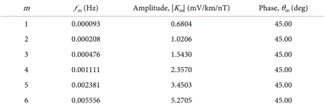
The transfer function amplitudes |Km| and phases θm for the uniform and layered Earth models, for the six frequencies in the synthetic magnetic data, are shown in Table 2 and Table 3.

(13)

[image:13.595.209.540.90.200.2]

Table 2. Transfer function for the uniform Earth model.

m ƒm (Hz) Amplitude, |Km| (mV/km/nT) Phase, θm (deg)

1 0.000093 0.6804 45.00

2 0.000208 1.0206 45.00

3 0.000476 1.5430 45.00

4 0.001111 2.3570 45.00

5 0.002381 3.4503 45.00

[image:13.595.208.539.234.347.2]

6 0.005556 5.2705 45.00

Table 3. Transfer function for the layered Earth model.

m ƒm (Hz) Amplitude, |Km| (mV/km/nT) Phase, θm (deg)

1 0.000093 0.2188 77.15

2 0.000208 0.4480 73.76

3 0.000476 0.8681 67.17

4 0.001111 1.5392 62.08

5 0.002381 2.5935 60.58

6 0.005556 4.6625 54.97

( )

6

(

)

1 m msin 2 m m m m

E t =

∑

₌ K A πf + Φ +θ (51)

Multiplying the |Km| and Am terms and adding the phases in (51) gives the electric field

( )

6

(

)

1 msin 2 m m m

E t =

∑

₌ E πf +ϕ (52)

with the six electric field waves as given in Table 4 for the uniform Earth model, and in Table 5 for the layered Earth model.

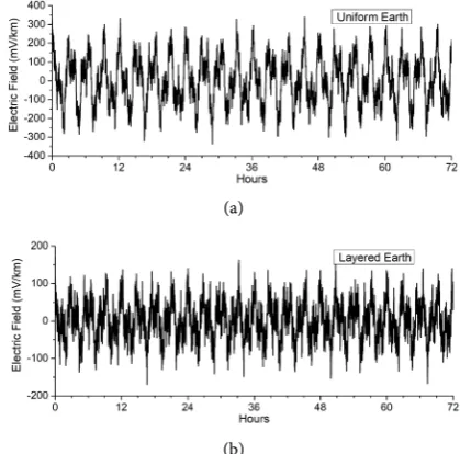
The synthetic geomagnetic field variation given by Equation (45) and Table 1 is shown in Figure 3. The exact geoelectric fields obtained from Equation (52) and Table 4 for the uniform Earth model and Table 5 for the layered Earth model are shown in Figure 4(a) and Figure 4(b), respectively. These waveforms provide analytic test cases that can be used to test the accuracy of numerical cal-culations. It is necessary to emphasize, referring to Section 2, that B expressed by Equation (45) with the parameter values given in Table 1 and shown in Figure 3 and E expressed by Equation (52) with the parameter values given in Table 4 or Table 5 and shown in Figure 4(a) or Figure 4(b) represent either Ex and By or −Ey and Bx.

(14)

[image:14.595.268.477.77.159.2]

Figure 3. Test magnetic field variation.

(a)

[image:14.595.266.476.195.402.2]

(b)

Figure 4. Exact electric fields. (a) For the uniform Earth model; (b) For the layered Earth model.

Table 4. Parameters of six electric field waves for the uniform Earth model.

m ƒm (Hz) Amplitude, Em (mV/km) Phase, ϕm (deg)

1 0.000093 136.0827 55.00

2 0.000208 91.85587 65.00

3 0.000476 46.29100 75.00

4 0.001111 40.06939 85.00

5 0.002381 27.60262 95.00

6 0.005556 18.44662 105.00

Table 5. Parameters of six electric field waves for the layered Earth model.

m ƒm (Hz) Amplitude, Em (mV/km) Phase, ϕm (deg)

1 0.000093 43.76735 87.15

2 0.000208 40.32327 93.76

3 0.000476 26.04161 97.17

4 0.001111 26.16634 102.08

5 0.002381 20.74819 110.58

[image:14.595.208.540.468.583.2] [image:14.595.207.539.616.736.2]

(15)

DOI: 10.4236/ijg.2019.1010053 944 International Journal of Geosciences (a)

[image:15.595.287.459.69.401.2]

(b)

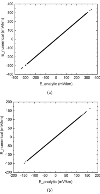
Figure 5. Comparison between numerical and analytic electric field values. (a) For the uniform Earth model; (b) For the layered Earth model.

Making a least-square fit to the data points in Figure 5(a) and Figure 5(b) as follows

numerical analytic

E =aE +b (53)

gives the values a = 0.999939118 (uniform), a = 1.000000135 (layered), b = 0.3250377 mV/km (uniform) and b = 0.042586 mV/km (layered). The good agreement between the numerical and analytic geoelectric fields shown by these numbers and correlation coefficients of 0.999999343 (uniform) and 0.999999989 (layered) confirm the accuracy of the numerical computation of geoelectric fields.

6. Calculation Using Tensor Transfer Functions

(16)

[image:16.595.284.466.71.196.2]

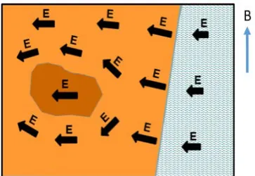
Figure 6. Deflection of electric fields by conductivity structure in the Earth.

In these cases the geoelectric fields and geomagnetic field variations are re-lated by a tensor transfer function in the frequency domain:

x xx xy x

y yx yy y

E K K B

     

=

     

      (54)

Thus the northward component of the geoelectric field, Ex, can be written

( )

x xx xy

E t =E t +E t (55)

where

( )

1

( )

{

( )

}

xx xx x

E t =F− _K f F B t _ (56)

( )

1

( )

{

( )

}

xy xy y

E t =F− _K f F B t _ (57)

Similarly, the eastward component of the geoelectric field, Ey, can be written

( )

y yx yy

E t =E t +E t (58)

where

( )

1

( )

{

( )

}

yx yx x

E t =F− _K f F B t _ (59)

( )

1

( )

{

( )

}

yy yy y

E t =F− _K f F B t _ (60)

It can be seen that these equations are just repeating the process used in the 1-D calculation. Therefore the numerical calculation method described in Sec-tion 4 can be used with the components of the tensor transfer funcSec-tion values and the verification process described in Section 5 can be used to test the calcu-lation of the geoelectric field parts given by (56), (57), (59) and (60).

In Equation (54) the minus sign in the relationship between Ey(ƒ) and Bx(ƒ) mentioned in connection with the 1-D transfer function K(ƒ) used in (14) is absorbed into the Kyx(ƒ) term. The Kxx(ƒ) and Kyy(ƒ) terms can be positive or negative depending on the conductivity structure. In an area where the structure is 1-D the tensor transfer function terms Kxx(ƒ) and Kyy(ƒ) are zero, and the diagonal terms are given by Kxy(ƒ) = K(ƒ) and Kyx(ƒ) = −K(ƒ).

7. Discussion

(17)

geoelectric fields. The accuracy of electric fields calculated for any particular site also depends on how well the Earth models for that location represent the Earth conductivity structure that is actually there. As mentioned above, the Earth has a complicated 3-dimensional conductivity structure and any Earth model used is inevitably an approximation to the real situation. One-dimensional models only take account of the variation of conductivity with depth, while 2-dimensional and 3-dimensional models attempt to represent some of the lateral variations in conductivity.

The Earth transfer functions used in the above calculations can either be ob-tained from models or directly from magnetotelluric (MT) measurements. The Earth conductivity models are also derived from MT measurements, so the two approaches should be equivalent. However, 2-D and 3-D models are derived by combining data from an array of MT sites so the Earth transfer function based on the model may not exactly reproduce the transfer functions measured at in-dividual MT sites.

MT measurements are not available everywhere. To provide Earth conductiv-ity information for areas with no MT measurements, zones with similar geologic structure have been identified and the MT results from a survey crossing part of a zone are applied to the rest of the zone. The geoelectric field can then be calcu-lated in each zone. These “piecewise” calculations then provide geoelectric field values across the whole region covered by a power grid and provide a simple approximate way of including Earth conductivity changes in the calculation of geomagnetically induced currents in a power network [13][22][29][30][31].

8. Conclusions

Calculation of the geoelectric fields produced during geomagnetic disturbances at the Earth’s surface is a key requirement for assessing the geomagnetic hazard to critical infrastructures such as power systems and pipelines.

The geoelectric field can be calculated by taking a Fourier Transform of a time series of magnetic field data, multiplying the magnetic field spectral compo-nents by the Earth transfer function to obtain the electric field spectrum, and then taking the inverse Fourier transform to obtain the geoelectric field in the time domain.

Accurate calculations require preprocessing (remove mean and trend and ta-per with a split cosine bell) of the magnetic field data as well as taking care of the placement of positive and negative frequency terms in the transform array and combining these with the appropriate Earth transfer function terms.

The numerical calculation process has been verified by testing with a synthetic magnetic field time series for which an exact analytic solution of the geoelectric field is available. Comparison of the calculated geoelectric fields with the analytic solution gives effectively perfect agreement (correlation coefficients better than 0.9999).

(18)

not a result of the computation process. Instead, they arise from uncertainties in the data used in the calculations. The sparsity of magnetic observing sites means that the magnetic field disturbances experienced by the parts of a power system, pipeline, or other affected infrastructure between observing sites are not neces-sarily accurately specified. Similarly, Earth transfer functions are based on mag-netotelluric surveys that only cover part of a network so they may not exactly represent the Earth conductivity structure throughout the entire system. When more magnetic data and Earth conductivity information become available they can be used with the methods described here to calculate better values of the geoelectric fields affecting critical infrastructure.

Acknowledgements

This work was performed as part of the space weather activities of the Public Safety Geoscience program at Natural Resources Canada. Contribution number: 20180404.

Conflicts of Interest

The authors declare no conflicts of interest regarding the publication of this pa-per.

References

[1] Turner, G. (2011) North Pole, South Pole. The Epic Quest to Solve the Great Mys-tery of Earth’s Magnetism. The Experiment, New York, 272 p.

[2] Campbell, W.H. (2003) Introduction to Geomagnetic Fields. 2nd Edition, Cam-bridge University Press, CamCam-bridge.

[3] Boteler, D.H., Pirjola, R.J. and Nevanlinna, H. (1998) The Effects of Geomagnetic Disturbances on Electrical Systems at the Earth’s Surface. Advances in Space Re-search, 22, 17-27.https://doi.org/10.1016/S0273-1177(97)01096-X

[4] Prescott, G.B. (1866) History, Theory and Practice of the Electric Telegraph. IV Edi-tion, Ticknor and Fields, Boston.

[5] Boteler, D.H. (2006) The Super Storms of August/September 1859 and Their Effects on the Telegraph System. Advances in Space Research, 38, 159-172.

https://doi.org/10.1016/j.asr.2006.01.013

[6] Gummow, R.A. (2002) GIC Effects on Pipeline Corrosion and Corrosion Control Systems. Journal of Atmospheric and Solar-Terrestrial Physics, 64, 1755-1764.

https://doi.org/10.1016/S1364-6826(02)00125-6

[7] Boteler, D.H. and Trichtchenko, L. (2015) Telluric Influence on Pipelines. In: Revie, R.W., Ed., Oil and Gas Pipelines: Integrity and Safety Handbook, Chapter 21, John Wiley & Sons, Inc., Hoboken, 275-288.https://doi.org/10.1002/9781119019213.ch21

[8] Boteler, D.H. (1994) Geomagnetically Induced Currents: Present Knowledge and Future Research. IEEE Transactions on Power Delivery, 9, 50-58.

https://doi.org/10.1109/61.277679

[9] Bolduc, L. (2002) GIC Observations and Studies in the Hydro-Québec Power Sys-tem. Journal of Atmospheric and Solar-Terrestrial Physics, 64, 1793-1802.

(19)

DOI: 10.4236/ijg.2019.1010053 948 International Journal of Geosciences 29-31 October 2003; Geomagnetically Induced Currents and Their Relation to Problems in the Swedish High-Voltage Power Transmission System. Space Weath-er, 3, S08C03.https://doi.org/10.1029/2004SW000123

[11] Guillon, S., Toner, P., Gibson, L. and Boteler, D. (2016) A Colorful Blackout. IEEE Power & Energy Magazine, 14, 59-71.

[12] Boteler, D.H. (2001) Assessment of Geomagnetic Hazard to Canadian Power Sys-tems. Natural Hazards, 23, 101-120.

[13] Viljanen, A., Pirjola, R., Wik, M., Ádám, A., Prácser, E., Sakharov, Y. and Katkalov, J. (2012) Continental Scale Modelling of Geomagnetically Induced Currents. Jour-nal of Space Weather and Space Climate, 2, A17.

https://doi.org/10.1051/swsc/2012017

[14] Viljanen, A., Pirjola, R., Prácser, E., Katkalov, J. and Wik, M. (2014) Geomagneti-cally Induced Currents in Europe. Modelled Occurrence in a Continent-Wide Pow-er Grid. Journal of Space Weather and Space Climate, 4, A09.

https://doi.org/10.1051/swsc/2014006

[15] Wik, M., Viljanen, A., Pirjola, R., Pulkkinen, A., Wintoft, P. and Lundstedt, H. (2008) Calculation of Geomagnetically Induced Currents in the 400 kV Power Grid in Southern Sweden. Space Weather, 6, S07005.

https://doi.org/10.1029/2007SW000343

[16] Boteler, D.H. (2015) The Evolution of Québec Earth Models Used to Model Geo-magnetically Induced Currents. IEEE Transactions on Power Delivery, 30, 2171-2178. [17] Love, J.J., Lucas, G.M., Kelbert, A. and Bedrosian, P.A. (2018) Geoelectric Hazard

Maps for the Mid-Atlantic United States: 100 Year Extreme Values and the 1989 Magnetic Storm. Geophysical Research Letters, 45, 5-14.

https://doi.org/10.1002/2017GL076042

[18] Kavanagh, E.R. (1974) Time Sequence Analysis in Geophysics. Third Edition, Univ. of Alberta Press, Edmonton, 492.

[19] Kaufman, A.A. and Keller, G.V. (1981) The Magnetotelluric Sounding Method. Methods in Geochemistry and Geophysics Vol. 15, Elsevier Scientific Publishing Com-pany, Amsterdam.

[20] Simpson, F. and Bahr, K. (2005) Practical Magnetotellurics. Cambridge University Press, Cambridge, 272 p.https://doi.org/10.1017/CBO9780511614095

[21] Chave, A.D. and Jones, A.G. (2012) The Magnetotelluric Method, Theory and Prac-tice. Cambridge University Press, Cambridge, 552 p.

https://doi.org/10.1017/CBO9781139020138

[22] Marti, L., Yiu, C., Rezaei-Zare, A. and Boteler, D. (2014) Simulation of Geomagnet-ically Induced Currents with Piecewise Layered-Earth Models. IEEE Transactions on Power Delivery, 29, 1886-1893.https://doi.org/10.1109/TPWRD.2014.2317851

[23] Bloomfield, P. (2000) Fourier Analysis of Time Series: An Introduction. John Wiley & Sons, New York, 2nd Edition, 269 p.

[24] Boteler, D.H. (2012) On Choosing Fourier Transforms for Practical Geoscience Ap-plications. International Journal of Geosciences, 3, 952-959.

https://doi.org/10.4236/ijg.2012.325096

[25] Bracewell, R.N. (1978) The Fourier Transform and Its Applications. Second Edition, McGraw-Hill Book Company, New York, 444 p.

(20)

DOI: 10.4236/ijg.2019.1010053 949 International Journal of Geosciences [27] Boteler, D.H., Pirjola, R.J. and Marti, L. (2019) Analytic Calculation of Geoelectric

Fields Due to Geomagnetic Disturbances: A Test Case. IEEE Access, 7, 147029- 147037. https://doi.org/10.1109/ACCESS.2019.2945530

[28] Boteler, D.H. and Pirjola, R.J. (1998) The Complex-Image Method for Calculating the Magnetic and Electric Fields Produced at the Surface of the Earth by the Auroral Electrojet. Geophysical Journal International, 132, 31-40.

https://doi.org/10.1046/j.1365-246x.1998.00388.x

[29] Viljanen, A. and Pirjola, R. (1994) On the Possibility of Performing Studies on the Geoelectric Field and Ionospheric Currents Using Induction in Power Systems.

Journal of Atmospheric and Terrestrial Physics, 56, 1483-1491.

[30] Viljanen, A., Pulkkinen, A., Amm, O., Pirjola, R., Korja, T. and BEAR Working Group (2004) Fast Computation of the Geoelectric Field Using the Method of Ele-mentary Current Systems and Planar Earth Models. Annales Geophysicae, 22, 101-113.https://doi.org/10.5194/angeo-22-101-2004

[31] Adám, A., Prácser, E. and Wesztergom, V. (2012) Estimation of the Electric Resis-tivity Distribution (EURHOM) in the European Lithosphere in the Frame of the EURISGIC WP2 Project. Acta Geodaetica et Geophysica Hungarica, 47, 377-387.