Title: Emergent Patterns of Population Genetic Structure for a Coral Reef Community Running title: Coral reef community genetics
Author list with address numbers: Kimberly A. Selkoe 1,2 Oscar E. Gaggiotti3, ToBo Laboratory4, Brian W. Bowen1, Rob J. Toonen1
Address List:
1. Hawai'i Institute of Marine Biology, University of Hawai'i, Kāne'ohe, Hawai'i 97644, USA 2. National Center for Ecological Analysis and Synthesis, 735 State St., Santa Barbara, California
93101, USA
3. School of Biology, Scottish Oceans Institute, University of St Andrews, St Andrews, Fife KY16 8LB, UK
4. Author names and affiliations listed in Appendix 1.
Abstract
What shapes variation in genetic structure within a community of co-‐distributed species is a central but difficult question for the field of population genetics. With a focus on the isolated coral reef ecosystem of the Hawaiian Archipelago, we assessed how life history traits influence population genetic structure for 35 reef animals. Despite the archipelago’s stepping stone configuration, isolation by distance was the least common type of genetic structure, and regional structuring (i.e., division of sites into genetically and spatially distinct regions) was most common, detected in 20 of surveyed species, and nearly all endemics and habitat specialists. IBD only occurred in four shallow, non-‐endemic invertebrates. Seven species displayed chaotic (spatially unordered) structuring, and all were non-‐endemic generalist species. Chaotic structure also associated with relatively high global FST. Pelagic larval duration (PLD) was not a strong predictor of variation in population structure (R2= 0.22), but accounting for higher F
ST values of chaotic and invertebrate species, compared to regional structuring and fish species, doubled the power of PLD to explain variation in global FST (adjusted R2=0.50). Multivariate correlation of eight species traits to six genetic traits highlighted dispersal ability and habitat specialization as strongest influences on genetics, but otherwise left much variation in genetic traits unexplained. Considering that the study design controlled for many sampling and geographical factors, the extreme interspecific variation in spatial genetic patterns observed for Hawai'i marine species may be generated by demographic variability due to species-‐specific abundance and migration patterns and/or seascape and historical factors.
KEYWORDS: Community genetics, stepping stone dispersal, chaotic genetic heterogeneity, Hawai'i , pelagic larval duration, marine connectivity
INTRODUCTION
The structuring of species into genetically distinct populations has many impacts on a species’ demography and evolution (Kokko & López-‐Sepulcre 2007). In turn, ecological and environmental factors influence population genetic structuring (Avise 2000; Storfer et al. 2007). Understanding linkages between ecological, genetic and environmental patterns is central to many current challenges in organismal biology and conservation (Taberlet et al. 2012). Uncovering generalities about these linkages requires comparison across multiple species, habitats and scales. Meta-‐analyses can test for meaningful relationships between genetic structuring and ecological traits across many species, but are hindered by the large number of possible confounding variables. In fact, an early finding of the rapidly expanding field of landscape genetics is that genetic structuring is highly species specific, influenced by the individual’s interaction with landscape features according to life history and demographic factors, such that generalities may be few (Manel et al. 2003). Marine systems are known for harboring diverse and often surprising spatial population genetic patterns (Selkoe et al. 2008). Here we characterize the variation in population genetic structure across species within a single marine community, which share a basic habitat array, environmental gradients and key study sampling design elements. Further, we examine whether life history traits associate with genetic patterns, perhaps pointing to mechanisms maintaining the diversity in genetic patterns across species.
There is great interest in determining what drives spatial patterns of population genetics for marine species, and the extent to which life history traits associate with particular types of structuring. Theory suggests that the scale and pattern of genetic structure reflects long-‐term rates of gene flow driven primarily by migration, drift and selection. A longstanding focus of the field of population genetics is the relationship of dispersal potential to gene flow, because dispersal is a difficult trait to study directly but central to many basic and applied questions in ecology. Across studies of marine species, dispersal traits show significant correlation to genetic structuring, albeit often only weakly (Bradbury et al. 2008; Weersing & Toonen 2009; Riginos et al. 2011; Selkoe & Toonen 2011; Faurby & Barber 2012), leaving open the question of whether the remaining variation in genetic differentiation between populations may be explainable by factors such as taxonomy, life history, sampling design or historical effects. Despite hundreds of single-‐species marine population genetics studies across the globe, it is still unclear whether stronger or more coherent links between genetic and life history traits might emerge if variables such as history, habitat array or taxonomy could be constrained.
combination of all these factors (Toonen & Grosberg 2011). The relative frequencies of these four types of genetic structuring and their main drivers are unknown for marine ecosystems.
The present study leverages recent genetic studies of Hawaiian coral reef species to examine the range of population genetic patterns across reef animals within a single community and investigate whether species traits co-‐vary with metrics and models of genetic structure. The geography of the Hawaiian Archipelago provides an especially tractable system in which to study marine population structure, because it is the remotest archipelago in the world, composed of a nearly linear 2,400 km long array of discrete habitat patches of islands, atolls and seamounts. Insofar as possible in a natural system, these factors constrain the patterns of population structure, connectivity across patches, and genetic history of populations (Fig. 1). We began by categorizing datasets for 37 diverse coral reef species sampled with standard genetic markers at >5 islands. Based on habitat array, we hypothesized that a stepping stone pattern of dispersal producing an isolation by distance pattern of spatial genetic structure would be prevalent. There are no obvious known physical barriers or strong oceanographic discontinuities that might lead to hierarchical genetic structuring. However, a precursor to this study found that locations of significant pairwise FST were highly variable across 27 species in Hawai'i, but occurred most commonly in the main Hawaiian Islands where islands are more closely spaced (Toonen et al. 2011).
Riginos et al. (2011) outlined two approaches to studying life history effects on population structure: planned multispecies comparisons using a common sampling regime and geography, and post-‐hoc compilation of published studies. This study represents a hybrid, in which compilation of raw genetic datasets for co-‐distributed species within a single discrete study region allowed a large degree of standardization. One would expect that by controlling for basic habitat array, environmental gradients and many shared historical influences, much of the noise in this relationship might be eliminated. In this way, more nuanced multivariate influences on gene flow could emerge, enhancing our understanding of the feedbacks between life history, ecology and genetics.
By comparing life history and genetic data across a broad taxonomic range of species, we hope to gain insights into the mechanisms that drive geographic population structuring in marine systems. We characterize variation in population structure across species in two ways. First, we constrain the question by theory, evaluating how the established models of genetic structuring are represented by the 39 species. Second, we use unconstrained ordination to determine natural divisions among the datasets based on a suite of genetic metrics of spatial structure. These two approaches are complimentary in that the first is using significance testing of how spatial distributions of genetic diversity fit with models, whereas the second is based on combinations of the metrics themselves, perhaps revealing additional divisions in the database which may not map well to the theory-‐based categories (i.e., if the values of the genetic metrics in each category show different ranges or variances).
et al. 2008; Kelly & Palumbi 2010; Riginos et al. 2011). We test each of these relationships here, and separately examine species with strong vs. weak genetic structuring, and Hawaiian endemics vs. widespread species, as endemism occurs at a high rate in Hawaii and could be associated with distinct genetic characteristics.
Methods
1. Dataset preparation format
Data sets were assembled primarily from collections made on NOAA expeditions throughout the Hawaiian archipelago from 2005 to 2012, and subsequent publications of mtDNA and nuclear DNA (usually microsatellite) data sets. Genetic datasets were contributed in ARLEQUIN format ( vers. 3.5.1.2, Excoffier & Lischer 2010), or an Excel format that allowed easy conversion to ARLEQUIN format. A
modified version of PGDSpider (vers. 2.0.5.1, Lischer & Excoffier 2012) was used to convert between file formats for genetic analyses. For coral species only, GENETIX ( vers. 4.05.2, Belkhir et al. 2002) was used to estimate and filter out clonal replicates within sites. ARLEQUIN files were modified to give all sites standardized four letter name codes and standardized ordering from SE to NW along the island chain. Because we have data at the scale of the island/atoll, we focus hypotheses at this spatial resolution. In most cases, allele/haplotype frequencies at adjacent islands are statically indistinguishable, indicating that island/atoll is an appropriate spatial scale for our study.
Any distinct sub-‐island or sub-‐atoll samples were kept separate, with distinct names, except when FST was statistically indistinguishable from zero, in which case sub-‐localities were lumped. Several species showed samples collected in the vicinity of Kona to be distinct from those near Hilo on Hawai'i Island, and Acanthaster planci showed two distinct populations at Pearl & Hermes Atoll.
2. Sampling filters
For inclusion in the analyses, a dataset required at least 5 sites sampled with at least 10 individuals per site. For datasets that meet these criteria, sites with fewer than 10 individuals were also excluded. We also analyzed results for a sample size minimum of because FST can be inflated at small sample size, and allele frequency estimates are less reliable for low frequency alleles at highly polymorphic loci. Using a minimum sample size of 20 individuals per site excluded 90 of 533 samples in the dataset using 10 or more samples per site (17% of samples). We comment below on how the two sampling filters affect results.
3. Summary statistics
2012) to choose the most appropriate mutational model in ARLEQUIN. SMOGD online calculator (Crawford 2010) was used to calculate DEST and effective alleles. GENODIVE’s K-‐means clustering was run for number of clusters (K) from 1 to N-‐2 using AMOVA based simulated annealing with 50,000 steps and 20 repeats. Cluster membership was examined to determine whether adjacent sampling sites clustered together, highlighting where genetic boundaries (i.e., genetic discontinuities) between regions might exist. Genetic boundaries were considered where AMOVA estimation of FCT across the boundary was statistically significant. The largest number of clusters of spatially discrete samples that returned significant FCT results with AMOVA was recorded. In most cases, this was K=2 or 3. In some cases, K-‐ means clustering showed slightly spatially-‐mixed clustering. For example if Midway, a Northwestern Hawaiian Islands (NWHI) site, grouped with the Main Hawaiian Islands (MHI) but otherwise MHI and NWHI sites were in two distinct clusters, a “spatially strict” versions of the clusters (e.g., Midway was placed in the NWHI cluster) were tested with AMOVA to confirm that FCT values were significant after the regrouping. This procedure was only used when 1-‐2 samples were geographically incongruent in the clustering results. Clusters made up of spatially mixed samples were considered evidence that genetic structuring was not regionally organized. Pairwise geographic distance between sites based on coordinates were generated using GENODIVE. Isolation by distance analyses were generated using linearized FST [FST/(1-‐FST)] vs. Euclidean distance. Significance testing was based on Mantel tests with 999 replicates performed in GENODIVE.
Nine species were represented by 2 datasets, one using a mtDNA marker and a second using one or more nuclear markers (e.g., microsatellite panels or nuclear intron sequence). Genetic summary statistics were calculated for each marker class independently and then compared to gauge congruence. The mtDNA dataset was preferentially chosen to represent the species in subsequent ordination analyses (which required one dataset per species to avoid double counting), except where sampling power of the nuclear dataset was superior, see results for details.
4. Categories of spatial genetic structure
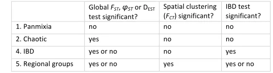
Based on the above summary statistics, datasets were placed into the following categories of spatial genetic structuring, summarized in Table 1:
(1) Panmixia -‐-‐ defined as a lack of spatial genetic structuring, indicated here when global FST, φST and DEST p>0.05, spatial groupings based on K-‐means clustering show FCT p>0.05, and IBD testing shows Mantel r p>0.05.
(2) Chaotic genetic heterogeneity -‐-‐ defined as genetic differentiation of samples with no apparent spatial organization, indicated here when global FST, φST and/or DEST p<0.05, but neither IBD nor any spatial clustering are statistically significant.
It is possible that a species could conform to more than one category in different regions of the archipelago. Most datasets could not be properly evaluated for this possibility due to limited sampling in remote portions of the archipelago. However, for every case of regional structure, we tested for the joint presence of IBD and regional groups. As illustrated by Meirmans (2012), IBD and hierarchical structure can be confounded. Hierarchical structure can mimic IBD when differentiation with regions is low and distant pairs are cross-‐regional comparisons, whereas IBD spatial autocorrelation can mimic hierarchical population structure if sampling is sparse and uneven. These scenarios were distinguished (albeit with low power in our case) using stratified Mantel tests in GENODIVE to permute the locations of populations within the clusters.
5. Clustering datasets by genetic summary statistics
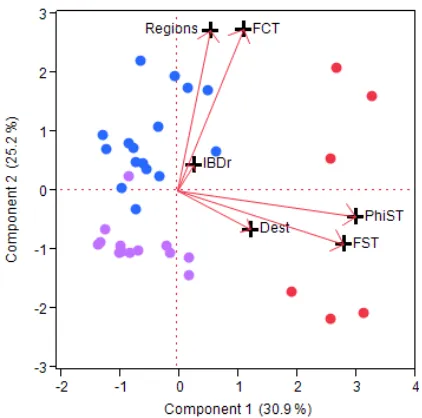
The above categorizations are based on labeling datasets according to their fit with existing models of genetic structure derived from genetic theory. The designations are based on the statistical significance at alpha=0.05 of a small number of genetic metrics. This approach ignores possibly useful information contained in the continuous range of values of the metrics themselves. It is also sensitive to sample size, which influences statistical significance. As an unconstrained alternative, we conducted a principle components analysis (PCA) with JMP ver. 10 (SAS). These included all genetic summary statistics (FST, φST, DEST, FCT, IBD r, and the number of genetic regions; Table S1) to find natural divisions in the datasets which are unconstrained by any pre-‐existing labels or theory. Genetic metrics were linearized and log transformed to homogenize scales prior to all analyses. Negative values of FST, φST and DEST were set to zero to avoid a confounding influence on ordinations. PCA allowed us to visualize the main trends in summary statistics, ascertain redundancy in summary statistics and visualize natural breaks or clusters of datasets by genetic traits.
6. Life History data
detritivore/sediments, invertivores and algivores vs. piscivores and planktivores) but provided no further insights to the analyses. Remaining life history categorizations were endemic to Hawai'i vs. non-‐ endemic, and free-‐floating eggs vs. attached to body or substrate. Higher taxonomic affiliation was also used as a categorical variable (fish vs. invertebrate and dolphin) representing fundamental but unspecified generalities that may tend to be shared across these highly diverse species, such as adult mobility, mutation rates or mating systems. A PCA using the 4 continuous variables and the 5 binary variables allowed us to assess the variation in the life history traits across species and visualize colinearities between life history traits, which were then confirmed with univariate linear regression or t-‐tests.
7. Redundancy analysis
Canonical analysis was used to assess how much the suite of life history traits explains the variation in genetic traits as a whole, and to visualize which traits most closely associate (Legendre & Legendre 2012). Redundancy analysis (RDA) is an ordination with regression; we used the package VEGAN in R for calculations. The genetic metrics (Y) are first transformed to Y’ by fitting the values to a linear regression of each life history trait (X). A PCA is then carried out on the Y’ values. Colinearity of life history traits was examined before proceeding, leading to the elimination of generation time, which was correlated to maximum length but generally measured with much less precision (OLS r=0.71). The genetic summary statistics used were the same as described above for PCA (Table S1). FST was used in place of φST for the 4 nuclear marker datasets as missing data is not allowed in the analysis. FST and φST were correlated (OLS r=0.71) but both were included in the analysis to reveal differences in their responses to species traits, as was our primary goal for the RDA instead of statistical hypothesis testing. All other genetic traits showed low colinearity. Two datasets with outlier FST values (FST>0.2) were removed (Cellana exerata and Chaetodon lunulatus) because outliers have disproportional influence on ordinations. We examined sampling factors as covariates in the analysis by performing a partial RDA with all factors (alleles, marker type, number of sites sampled, recent arrival species), but no effects were found. Adjusted R2 was calculated following the Ezekiel method (Legendre & Legendre 2012). The RDA triplot provided guidance on where to concentrate tests of particular associations of life history and genetic traits (i.e., it showed which traits have the strongest associations) to avoid large ratio of alternative models to sample size (Burnham & Anderson 2002).
8. Linear models of genetic differentiation
RESULTS
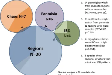
1. Genetic Categorizations
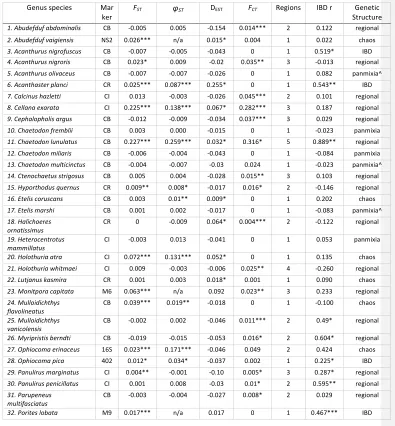
Datasets were divided into all four possible categories of genetic structuring: regional, IBD, chaotic and panmictic (Fig. 2, Table S1). Among species sampled with two marker types, five of the nine showed congruent categorization of both datasets. The remaining four species all had one dataset with a low number of alleles that showed panmixia, and the other dataset had a high number of alleles that showed structuring. The association of low polymorphism with panmixia was the most prominent sampling factor associated with placement of a dataset into one of the four categories (Table S2). To avoid double counting in analyses requiring one dataset per species, we selected the dataset with the more polymorphic marker(s) because of its greater statistical power. For the congruent pairs, the mtDNA datasets were preferentially selected to increase consistency in marker type across datasets. Regional grouping was the most common type of spatial genetic structure, observed in 20 of the 37 species. Eight species showed support for two spatial regions, eight for three regions, three for four regions and one for five regions (Table S1). In some cases, “regions” comprised only one sample separated from others by a significant genetic break. In all but three of these species, hierarchical AMOVA showed no evidence of significant finer scale structuring within regions (i.e., significant FSC values; exceptions were Stenella longirostris and Montipora capitata). Although ten of the 20 regionally structured species showed significant overall IBD results (uncorrected p<0.05), none showed a significant stratified Mantel test, which would indicate IBD within regions. Thus, these IBD signals are likely an artifact of the regional structuring (the increased mean pairwise FST across regions compared to within regions), although for a minority, the stratified Mantel test may have lacked power to detect a true within-‐region IBD signal. Interestingly, twelve of the 20 regionally structured species showed global FST values not significantly different from zero. Add assessment of sampling gaps contributing to significance of IBD results.
Only four species were categorized as IBD, because they showed significant IBD without any regional structuring. One of these, Acanthurus nigrofuscus, had a very weak signal (p=0.05) and most pairwise FST <0. The other three species classified as IBD datasets were invertebrates: a sea star (Acanthaster planci), a coral (Porites lobata) and a brittlestar (Ophiocoma pica).
Seven species categorized as chaotic showed highly significant global differentiation among sample sites and many significant pairwise FST values, but with no obvious spatial organization. However, one of these species, the brittlestar Ophiocoma erinaceus, showed a nearly significant IBD test (r=0.42, p=0.07) and nearly significant test for 2 regions (FCT=0.049, p=0.15) that might have gained significance with more specimens. Two of the chaotic datasets yielded FST with p>0.05, but DEST and/or φST were highly significant.
Changing minimum sample size from 10 or more individuals per location to 20 or more affected the categorization of only 1 dataset (Chaetodon miliaris lost four sites and switched from panmictic to regionally structured). Several other species lost enough sites to be excluded from analysis.
2. Ordinations of genetic traits and life history traits
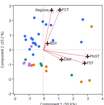
The six genetic summary statistics (FST, φST, DEST, FCT, number of significant regions, IBD fit) showed only moderate to low colinearity. The most correlated values were φST and FST (OLS r=0.71). DEST was uncorrelated with φST and FST. A PCA using these six genetic summary statistics showed two datasets (limpet C. exerata and butterflyfish C. lunulatus) to be outliers to the rest because their values of φST, FST DEST and FCT were much larger than the others (e.g., FST>0.2 vs. <0.09, Table S1). These two datasets were removed from all further analyses and the PCA was repeated to lessen the influence of skew on the analysis. The first 4 PCs showed eigenvalues>1 (Fig. 3a). The first PC, which showed high loadings for both φST and FST, separated out six datasets for which differentiation among sites is largest (e.g., FST>0.02; red markers in Fig. 3a). PC2 separated most of the datasets with 1 region and high FCT values (purple in Fig. 3a) from those with multiple regions and low FCT values (blue in Fig. 3a). PC3 was correlated with IBD r and PC4 with DEST. To show how the four categories of genetic structuring map to the PCA results, the biplot is recolored in Fig. 3b; it indicates that chaotic and IBD spatial organization are not clustered into a small range of values of FST or φST.
A PCA of the life-‐history traits show that species have diverse combinations of traits instead of a few clusters of associated types (see Fig. S1 for biplot and more detail). Pairwise linear regressions testing revealed two notable apparent correlations among life history traits. As previously known, Generation Time and Maximum Length positively associate (OLS R2=0.52, p<0.0001). We excluded Generation Time from the RDA analysis due to colinearity. Also, fishes showed significantly broader depth ranges than invertebrates (R2=0.30, p<0.0001) but both were retained in the RDA as correlation was weak. The biplot shows that the genetic types contain a mixture of life history traits, but some tend to be absent from certain quadrants: for PC1 v PC2, chaotic datasets tend to be in the upper left (all were non-‐endemic and habitat generalists), panmictic datasets in the upper half (broad and deep depth ranges and mostly fish), and IBD datasets in the lower half (shallow and invertebrate), whereas regional species are widely distributed over the plot.
4. Redundancy analysis of life history and genetic traits
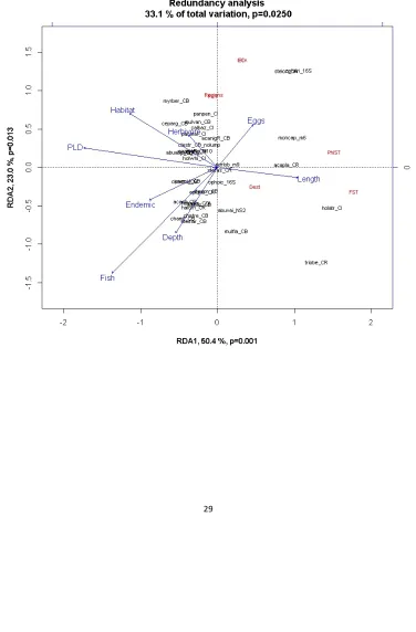
The multivariate linear relationship between eight life history and six genetic traits was significant but not strong (R2=0.35, adj. R2=0.11, p=0.037). When φ
ST is excluded to reduce redundancy with FST, R2 is unchanged but p=0.055. In both cases, all eigenvectors were <1 indicating lack of principle component interpretability. The triplot is nonetheless useful for visualizing which life history traits associate with genetic traits (Fig. 4). Three traits (PLD, Fish, Habitat) are located near the edges indicating strongest explanatory power. A reduced model with only these 3 traits raises the adjusted R2 (R2=0.22, adj. R2=0.15, p=0.001). Three genetic traits (Regions, D
The vector for IBD is opposite the trajectory of Fish, Endemic and Depth range, indicating negative relationships of these traits to stepping stone dispersal. As in Fig. 3a, the plot separates the species with strong differentiation on the right side, away from the majority of other datasets. These species are a shark, a dolphin, a sea cucumber, a coral, a sea star and a brittlestar, a group encompassing all 3 types of spatial genetic structuring.
5. Linear modeling of genetic traits
The RDA indicates that Fish, Endemic and Depth have strong negative impacts on IBD r. A comparison of multivariate GLM models for these three traits and their interactions showed the most parsimonious model of IBD r includes Endemic and Depth only (adj. R2=0.22, p=0.006); shallow, non-‐endemic invertebrates show stronger IBD patterns. Maximum depth, not minimum depth drives the correlation with depth range.
A linear fit of PLD vs. FST was highly significant (OLS R2=0.45, p<0.0001, Fig. 5), but when the two species (shark and dolphin) that lack larval development are excluded, the fit drops (R2=0.19, p=0.012). The fit strengthens slightly (R2=0.22) without the 6 panmictic datasets, for which F
ST is less informative because it is measured with larger error and is likely an artefact of low marker polymorphism for many of the datasets (Table S2)..
For this subset of 27 non-‐panmictic species with PLD>0, a comparison of multivariate GLM models based on AICc showed that a model with Fish and PLD is more parsimonious than a model of PLD alone (adj. R2=0.31, p=0.044, ΔAIC
c=2.5, Table 4). Adding Fish improved the fit because invertebrates have a higher intercept than fishes due to their generally higher FST values. Adding in the other 8 species traits as additional factors does not improve the model (only individual additions were tested to minimize number of models compared). However, adding an indicator of whether the dataset shows spatially organized structure (regional or IBD) or disorganized structure (chaotic) as a covariate improves the model significantly (adj. R2=0.50, p<0.0001, ΔAIC
c=6.8, Table 4). The model improvement occurs because chaotic datasets have a higher FST values on average and thus a higher intercept for PLD vs. FST.
Categorization of datasets as regional or chaotic was made based on the p value of FCT in a hierarchical AMOVA, which shows no correlation with FST (R2=0, p=1.0). With the two direct developers (PLD=0) included, the fit of this model is boosted (adj. R2=0.65). Interactions were not significant and thus excluded from the best fit model.
The 10 endemics show no relationship between PLD and FST, although all endemic PLD values are fairly large (PLD>23 days). No species traits significantly explain FST for the endemics. Excluding endemics from the non-‐panmictic, PLD>0 group, results in the same best fit model, but with higher explanatory power (adj. R2=0.58, Table 4).
We examined how GLM models explain variation in φST for the mtDNA datasets compared to those for FST. Fish and structure type (i.e., spatially organized vs. disorganized) without PLD best explained φST for the PLD>0 non-‐panmictic set of species (adj. R2=0.55, p<0.002). φ
ST also shows no relationship to PLD for endemics, but shows a highly significant positive relationship to both maximum length and herbivory for endemics (adj. R2=0.66, p=0.009). D
Discussion
It is well known that marine species exhibit extensive variation in their genetic patterns that is poorly predicted by ecological or species traits. By focusing on a single isolated region with a simplistic habitat array and calculating genetic metrics in a standardized way from raw data of many species, we investigated the extent to which variation in genetic patterns is constrained across species using two complimentary approaches. The dual approaches help illuminate the extent to which our assessment is sensitive to the chosen metrics, categories, and statistical framework. First, the PCA analysis focused on the strength of genetic differentiation and the spatial scale of structuring (i.e., number of regions), and revealed 3 clusters within the species set: single region/low differentiation, multi-‐regional/moderate differentiation and a small number of high differentiation species with a mix of single and multiple regions. Second, the categorization of the datasets into four a priori types focused primarily on the spatial organization of the structuring and not the strength of differentiation (i.e., regional, IBD, chaotic and panmictic). Comparison of these two approaches revealed that species with strongest structuring show diverse spatial organization of structuring and likely a diversity of causes for that high structuring. Life history analyses revealed that chaotic species were all non-‐endemic and habitat generalists, IBD occurred for four shallow invertebrate habitat generalists, regionally structured species showed a variety of life history associations, and panmixia was mostly limited to fishes with broad and deep depth ranges or associated with low allelic diversity indicating low statistical power. Polymorphism creates precision much the way increasing the number of samples would (Kalinowski 2002).
Regional Boundaries across the Archipelago
endemics and all habitat specialists were regionally structured (except a few cases of panmixia). Both groups are more likely to have variable abundance across the chain due to spatially varying micro-‐ habitats, supporting this cause for regional structuring. This phenomenon begs for marine population genetic studies to carefully consider sampling design and run simulations to test effects of sampling factors on results. Additional factors and analysis approaches might add insight to the current results. For example, if ocean currents are important drivers of gene flow, the seasonal timing of larval dispersal, and other larval traits for which we were unable to find data, may help generate variation in genetic structuring across these species. We will explore the relative roles of history, oceanography, sampling and habitat factors in generating the observed variation in genetic patterns across species in future studies.
Statistical considerations of characterizing spatial genetic structure
Our dataset proved to be a good example of the ‘trouble with isolation by distance,’ described recently by Meirmans (2012). Nine datasets showed significant test results for IBD that on closer examination were driven only by regional structuring, evident both by examining site membership of data points on the IBD plot and by a stratified Mantel test. Our algorithm for categorizing a dataset by its spatial genetic structuring was inspired by this study, and at least in the case of marine species, it appears that understanding whether the dataset is spatially auto-‐correlated, regionally structured or chaotically structured is an important first step to interpreting population genetic analyses. Meirmans (2012) found that 70% of a sample of studies testing for IBD found it. These were mostly terrestrial or aquatic studies. It is already known that marine species show much lower rates of IBD, and in this study, despite an uncommonly clear-‐cut stepping stone habitat array, only 10% of species showed IBD. It is unlikely sampling gaps biased the categorization of datasets as IBD vs. regionally structured, as the average number of samples, number of sites in the MHI, NWHI and whole chain, and the size of the largest sampling gap were nearly identical for the two groups (Table S2). However, IBD datasets tended to have slightly larger effective number of alleles than regional datasets (4.1 vs. 3.6; Table S2). Similarly, chaotic and panmictic datasets
Many species showed global estimates of FST and φST near zero despite strong regional structuring. Despite the fact that island-‐scale differentiation (global FST) correlated with PLD, many species in the highest PLD category showed 2 or 3 genetically distinct regions, perhaps indicating that regional boundaries are not caused by dispersal related processes and instead may be a product of historical events (Marko 2004) and/or local adaptation. The K-‐means clustering approach to guide hierarchical AMOVA has not been widely used, but is more sensitive than a priori designation of groups. While it has the potential to uncover large-‐scale structure that is missed by other approaches (e.g., Kelly & Eernisse 2007; Díaz-‐Ferguson et al. 2010), it is also possible that the approach has inflated type 1 error. Regional, taxonomic and life history variation in the correlation of PLD and FST
(Broquet & Yearsley 2012), which may occur even in species with extremely long pelagic developmental periods (Iacchei et al. 2013).
The correlation of PLD and FST (R2=0.22 for species with pelagic larvae) was lower than the value for a global sample of studies (R2~0.30) derived from a variety of spatial scales, habitat configurations, regions and environmental settings (Selkoe & Toonen 2011). Furthermore, our sample of φST showed no significant relationship to PLD, instead correlating just with taxon, consistent with φST having higher sensitivity to demographic history and mutation than FST (Bird et al. 2009, 2011; Meirmans & Hedrick 2011). For any isolated marine habitat, retention strategies are crucial to persistence, but PLD may be less indicative of realized dispersal distance in this extremely isolated ecosystem compared to other places (but see Schultz & Cowen 1994; Robertson 2001). This possibility is supported by two additional insights. First, endemics, which may be more dependent on larval retention for persistence than widespread species, showed no relationship of FST to PLD. However, all endemics in the study have PLD>20 days, after which the linear relationship saturates. Thus, retention of larvae may not be highly related to the mean PLD in this setting. Second, comparison of the correlation strength for Hawai'i to that found in other regions shows that the PLD v. FST correlation is relatively weak in Hawai'i (Fig. 7). Aside from poor correlation of PLD and dispersal distance, there are many other factors that can decouple PLD and FST values. One recent focus has been the influence of coalescent time on FST, such that holding coalescent time constant should improve PLD vs. FST correlation (Dawson et al. 2014). An anlysis using hierarchical approximate Bayesian computation (Hickerson & Meyer 2008; Beaumont 2010) of our dataset indicate nearly uniform timing and rate of expansion following the last glacial maximum (Chan et al. in prep). Therefore, we conclude that different coalescent histories are likely not driving variation in genetic patterns of these species. Contrary to claims that comparisons among synchronously diverging co-‐distributed (SDC) species “consistently evince higher gene flow in species with higher dispersal potential” (Dawson 2014), results from SDC taxa in Hawai'i (and previous global analyses; Selkoe and Toonen 2011) mandate a more nuanced treatment of the many forces impacting the population genetics of marine species.
We found that fishes show less structure and less organized structure than invertebrates. This point has not been previously highlighted, but the pattern is evident in other marine datasets (Carpenter et al. 2011; Toonen et al. 2011; Selkoe & Toonen 2011). Compared to invertebrates, fishes generally are more capable of behaviors that promote dispersal, and adult and juvenile migration is possible (Eble et al. 2011; Poortvliet et al. 2013). In addition, we found that species with deeper depth ranges tend to show less structuring than shallow species ( also see Etter et al. 2005; Kelly & Palumbi 2010; Gaither et al. 2012; Andrews et al. 2014), perhaps because shallow habitat is smaller in total area, harder for larvae to intercept, and subject to more frequent disturbance, contributing to higher rates of genetic drift. The reason that only shallow invertebrates showed IBD may be due to the double constraint of limited dispersal ability and smaller habitat patch sizes.
variation in spatial patterns of genetic differentiation will bring new insights to this line of inquiry (Lowe & Allendorf 2010; Marko & Hart 2011a; b).
Multivariate estimates of the covariation of species and genetic traits
Canonical analysis of how 8 species traits associated with genetic traits revealed that PLD, taxonomy (fish vs. invertebrate) and habitat specialization had the strongest influences on FST, φST and IBD fit, but overall explanatory power was low. Our use of RDA to uncover associations of life history and genetic traits followed a similar study of 27 co-‐distributed high-‐alpine plants of the European Alps (Meirmans et al. 2011). That study used AFLP data to generate 8 genetic summary statistics describing spatial genetic diversity, paired with 6 species traits related to dispersal and habitat preference. The 6 species traits together explained a very similar fraction of variation in genetic traits relative to our finding (R2=0.30, adj. R2=0.17). Considering the diversity of ecological, organismal, and historical factors that can impact the distribution of genetic diversity, the authors interpreted this as a large fraction. Our dataset included a wider diversity of species in terms of life history and taxonomy. Interestingly, Meirmans et al. (2011) analysis showed the same qualitative main results we report here. First, FST was the most strongly predicted trait, and was driven by dispersal factors. Plants with multiple dispersal modes showed higher gene flow, similar to our finding that fishes, which can disperse both as adults and larvae, show higher gene flow than invertebrates. Second, Mantel r was the only other strongly predicted genetic metric aside from FST in both studies, and rather than associating with dispersal factors as would be expected, it was best predicted by habitat factors (soil type for plants, depth range for coral reef species). Historical factors (i.e., size and distribution of refugia) may drive both the depth and soil type effects, and retrospective analyses using coalescent models are needed to distinguish ancient connectedness from contemporary gene flow. A final similarity to Miermans et al. (2011) is that Jost’s DEST showed no correlation with life history or other genetic traits, thus providing little insight in either context. Despite the study design to limit sources of natural variance, the species included in this study showed great variation in genetic structure, and species traits were not highly predictive of that variation. Two of the species showed extremely high spatial structuring relative to all others, one regionally structured and one chaotically structured. Their exclusion from the analysis serves only to weaken the link between genetic variation and species traits. In sum, the question of what maintains the extreme diversity in spatial genetic patterns across marine species remains largely unanswered by this study, but is narrowed by the finding that it persists despite controlling for sampling design, marker type, habitat array, major environmental and oceanographic gradients and recent history to a greater extent than possible in meta-‐analyses of published works. Even within a single reef community, life history of marine species is extremely diverse and likely drives high diversity of demographic and genetic patterns. Genetic diversity is a crucial foundation for biodiversity, with demonstrated influence on fitness, persistence, species diversity, and ecosystem functioning (reviewed in Hughes et al. 2008; Taberlet et al. 2012). There is great interest in integrating population genetics into community ecology to understand the forces controlling community assembly and species interactions (Avise 2000; Wares 2002; Cavender-‐ Bares et al. 2009). Continuing to characterize the forces controlling spatial genetic structure in more marine and terrestrial communities and regions is an important first step.
Funding was provided to K. Selkoe and R. Toonen by the National Science Foundation (BioOCE Award Number 1260169) and the National Oceanic and Atmospheric Administration (NMSP MOA#2005-‐ 008/66882). O. Gaggiotti was supported by the Marine Alliance for Science and technology for Scotland (MASTS). We are grateful to Heidi Lischer for modifying the software PGDSpider on our request, to the following for contributing ideas and feedback: Eric Crandall, Mary Donovan, and Alan Friedlander; and to the following for contributing raw data: Giacomo Bernardi, Mathew Craig, Marina Ramon, and Nicholas Whitney.
Author Contributions
KAS, RJT & OG designed research, KAS performed research, KAS analyzed data and KAS, RJT, OG and BB wrote the paper. Tobo Laboratory authors contributed data and analyzed data.
Data Accessibility
Dryad DOI, scripts, datasets
Literature Cited
Arnaud-‐Haond S, Vonau V, Rouxel C, Bonhomme F, Prou J, Goyard E, Boudry P (2008) Genetic structure at different spatial scales in the pearl oyster (Pinctada margaritifera cumingii) in French Polynesian lagoons: beware of sampling strategy and genetic patchiness. Marine Biology, 155, 147–157. Avise JC (2000) Phylogeography: The History and Formation of Species. Harvard University Press,
Cambridge, MA.
Baums ILB, Miller M, Hellberg ME (2006) Geographic variation in clonal structure in a reef-‐building Caribbean coral, Acropora palmata. Ecological Monographs, 76, 503–519.
Beaumont MA (2010) Approximate Bayesian Computation in Evolution and Ecology. Annual Review of Ecology, Evolution, and Systematics, 41, 379–406.
Belkhir K, Borsa P, Chikhi L, Raufaste N, Bonhomme F (2002) GENETIX 4.04, logiciel sous WindowsTM pour la genetique des populations. Laboratoire Genome, Populations, Interactions, CNRS UMR 500, Universite de Montpellier II, Montpellier, France.
Bird CE, Karl SA, Toonen RJ (2009) Detecting and Measuring Genetic Differentiation . Phylogeography and Population Genetics in Crustacea, 19, 31–55.
Broquet T, Yearsley JM (2012) Genetic drift and collective dispersal can result in chaotic genetic patchiness. Evolution, 1660–1675.
Burnham KP, Anderson DR (2002) Model Selection and Multimodel Inference: a Practical Information-‐ Theoretic Approach. Springer-‐Verlag, New York.
Carpenter KE, Barber PH, Crandall ED, Ablan-‐Lagman MCA, Mahardika GN, Manjaji-‐Matsumoto BM, Juinio-‐Meñez MA, Santos MD, Starger CJ, Toha AHA (2011) Comparative Phylogeography of the Coral Triangle and Implications for Marine Management. Journal of Marine Biology, 2011, 1–14. Cavender-‐Bares J, Kozak KH, Fine PV a, Kembel SW (2009) The merging of community ecology and
phylogenetic biology. Ecology letters, 12, 693–715.
Craig M, Eble J, Bowen B, Robertson D (2007) High genetic connectivity across the Indian and Pacific Oceans in the reef fish Myripristis berndti (Holocentridae). Marine Ecology Progress Series, 334, 245–254.
Craig MT, Eble J a., Bowen BW (2010) Origins, ages and population histories: comparative
phylogeography of endemic Hawaiian butterflyfishes (genus Chaetodon). Journal of Biogeography, 37, 2125–2136.
Crawford N (2010) SMOGD: software for the measurement of genetic diversity. Molecular ecology resources, 10, 556–557.
Darriba D, Taboada GL, Doallo R, Posada D (2012) jModelTest 2: more models, new heuristics and parallel computing. Nature Methods, 9, 772–772.
Dawson MN, Hays C, Grosberg RK, Raimondi PT (2014) Dispersal potential and population genetic structure in the marine intertidal of the eastern North Pacific. Ecological Monographs, in press. Díaz-‐Ferguson E, Haney R a, Haney R, Wares JP, Wares J, Silliman BR, Silliman B (2010) Population
genetics of a trochid gastropod broadens picture of Caribbean Sea connectivity. PloS one, 5. Etter RJ, Rex MA, Chase MR, Quattro JM (2005) Population differentiation decreases with depth in deep-‐
sea bivalves. Evolution; international journal of organic evolution, 59, 1479–91.
Excoffier L, Lischer HE (2010) Arlequin suite ver 3.5: a new series of programs to perform population genetics analyses under Linux and Windows. Molecular ecology resources, 10, 564–7. Faurby S, Barber PH (2012) Theoretical limits to the correlation between pelagic larval duration and
population genetic structure. Molecular ecology, 21, 3419–3432.
Foster NL, Paris CB, Kool JT, Baums IB, Stevens JR, Sanchez JA, Bastidas C, Agudelo C, Bush P, Day O, Ferrari R, Gonzalez P, Gore S, Guppy R, McCartney MA, McCoy C, Mendes J, Srinivasan A, Steiner S, Vermeij MJA, Weil E, Mumby PJ (2012) Connectivity of Caribbean coral populations:
Galindo HM, Pfeiffer-‐Herbert AS, McManus MA, Chao Y, Chai F, Palumbi SR (2010) Seascape genetics along a steep cline: using genetic patterns to test predictions of marine larval dispersal. Molecular ecology, 19, 3692–707.
Hedgecock D, Pudovkin AI (2011) Sweepstakes Reproductive Success in Highly Fecund Marine Fish and Shellfish: A Review and Commentary. Bulletin of Marine Science, 87, 971–1002.
Hedrick PW (2005) A standardized genetic differentiation measure. Evolution, 59, 1633–8.
Hickerson MJ, Meyer CP (2008) Testing comparative phylogeographic models of marine vicariance and dispersal using a hierarchical Bayesian approach. BMC evolutionary biology, 8, 322.
Hughes AR, Inouye BD, Johnson MTJ, Underwood N, Vellend M (2008) Ecological consequences of genetic diversity. Ecology letters, 11, 609–23.
Johnson MS, Black R (1982) Chaotic genetic patchiness in an intertidal limpet, Siphonaria sp. Marine Biology, 70, 157–164.
Kalinowski ST (2002) How many alleles per locus should be used to estimate genetic distances? Heredity, 88, 62-‐65.
Kelly RP, Eernisse DJ (2007) Southern hospitality: a latitudinal gradient in gene flow in the marine environment. Evolution, 61, 700–7.
Kelly RP, Palumbi SR (2010) Genetic structure among 50 species of the northeastern Pacific rocky intertidal community. PloS one, 5, e8594.
Kokko H, López-‐Sepulcre A (2007) The ecogenetic link between demography and evolution: can we bridge the gap between theory and data? Ecology letters, 10, 773–82.
Legendre P, Legendre L (2012) Numerical Ecology. Elsevier B.V., Amsterdam.
Lischer HEL, Excoffier L (2012) PGDSpider: an automated data conversion tool for connecting population genetics and genomics programs. Bioinformatics, 28, 298–9.
Long (I'll fill this in)
Lowe WH, Allendorf FW (2010) What can genetics tell us about population connectivity? Molecular ecology, 19, 3038–51.
Manel S, Schwartz MK, Luikart G, Taberlet P (2003) Landscape genetics: combining landscape ecology and population genetics. Trends in Ecology & Evolution, 18, 189–197.