Farms, Pipes, Streams and Reforestation:
Reasoning about Structured Parallel
Processes using Types and Hylomorphisms
David Castro, Kevin Hammond, Susmit Sarkar
School of Computer Science, University of St Andrews, St Andrews, Scotland {dc84, kh8, ss265}@st-andrews.ac.uk
Abstract
The increasing importance of parallelism has motivated the cre-ation of better abstractions for writing parallel software, including structured parallelism using nested algorithmic skeletons. Such ap-proaches provide high-level abstractions that avoid common prob-lems, such as race conditions, and often allow strong cost mod-els to be defined. However, choosing acombinationof algorithmic skeletons that yields good parallel speedups for a program on some specific parallel architecture remains a difficult task. In order to achieve this, it is necessary to simultaneously reason both about the costs of different parallel structures and about the semantic equiva-lences between them. This paper presents a new type-based mecha-nism that enables strong static reasoning about these properties. We exploit well-known properties of a very general recursion pattern, hylomorphisms, and give a denotational semantics for structured parallel processes in terms of these hylomorphisms. Using our ap-proach, it is possible to determine formally whether it is possible to introduce a desired parallel structure into a program without al-tering its functional behaviour, and also to choose a version of that parallel structure that minimises some given cost model.
Categories and Subject Descriptors D.3.2 [Language Classifi-cations]: Concurrent, distributed, and parallel languages; D.1.3 [Programming Techniques]: Parallel Programming; D.3.1 [For-mal Definitions and Theory]: Semantics
Keywords Parallelism, type-systems, hylomorphisms, term rewrit-ing systems.
1.
Introduction
Providing suitable abstractions to allow reasoning about paral-lelism is crucial to allow safe exploitation of increasingly par-allel hardware. To date, however, there has been only a limited amount of work on this issue: the static analysis community has been concerned primarily with provable safety, whereas the paral-lelism community has been concerned primarily with practically demonstrable performance. In order to meet both demands, it is necessary to simultaneously consider boththe functionaland the extra-functional properties of a parallel program. This paper
presents a new approach, a type-based mechanism that enables us to reason about the safe introduction of parallelism, while also pro-viding a good abstraction to reason about cost. This mechanism exploits strong program structure in the form of structured parallel processes [3], combined with properties ofhylomorphisms[22].
1.1 Motivating Example
We introduce our approach using a simple example,image merge, which merges pairs of images taken from an input stream. We start with a simple structure, where the functionality of the program is split into two functions:mark, which marks the pixels that are to be merged; andmerge, whichreplaces these pixels. A straightforward implementation would use the usualmapconstruct on lists:
imgMerge : List(Img×Img) → List Img imgMerge = map(merge ◦ mark)
Given two well-known algorithmic skeletons, farm for parallel replication andpipelinefor parallel composition, even this simple example presents several alternative parallelisations, including:
imgMerge1 = farmn(fun(merge◦mark))
imgMerge2 = farmn(fun mark)kfarmm(fun merge) imgMerge3 = farmn(fun merge)kfun mark
. . .
wherefun(f) encapsulates sequential functionality andp1 k p2
represents a 2-stage parallel pipeline. All these implementations are semantically equivalent toimgMerge: they differ only inhow the computation is performed, and thus in its performance. In this paper, we will describe a type system that annotates top-level types with the (parallel) structure, and will use this to au-tomaticallychoose a parallelisation. For example, if we define
IM(n,m) = FARMn(FUN A)kFARMm(FUN A), we could write:
imgMerge : List(Img×Img) 7−IM−−−−−(n,m→) List Img imgMerge = map(merge ◦ mark)
The type system will then automatically selectimgMerge2.Rather
than manually changing the definition ofimgMergeto a parallel one, we can simply change the type annotationIM(n,m)and
au-tomatically introduce the corresponding parallel implementation. The soundness of the type system provides strong static guarantees that the resulting program is functionally equivalent to the original form. Moreover, we can even use the type system toinferpart of this parallel structure. For example, if we defineIM1(n,m) = k
FARMm andIM2(n,m) =min cost( kFARMm ), then the parts ofIM1that are denoted by will be filled with the simplest possible
(parallel) structure and the parts ofIM2that are denoted by will be
1.2 Contributions
The paper makes the following main novel contributions:
•We define a denotational semantics for a set of well-known al-gorithmic skeletons, that cover a good range of parallel pro-grams, in terms ofhylomorphisms(Section 3).
•We identify semantic equivalences of parallel processes built using nested algorithmic skeletons as part of atype systemthat allows us to rationally choose a suitable parallel structure for a program (Section 4).
•We introduce a decision procedure for such semantic equiv-alences, based on reintroducing intermediate data structures, “reforestation”, rather than the more common approach of eliminating them for efficiency reasons, “deforestation”. This enables the type system to introduce parallelism in a semi-automated and sound way (Section 5).
2.
Type Preliminaries
Our denotational semantics is phrased in a standard categorical lan-guage [10], with a category representing amodel of computation, the objects of that category representingtypes, the morphisms rep-resentingprograms, andendofunctorsfrom the category to itself representing type constructors. In line with common practice [34], we will work in the category ofpointed complete partial orders (CPO). Our type language is entirely standard:
A,B ::= τ|1|A+B|A×B|A→B|F A|µF We assume no knowledge about the definition of anatomic type (τ), but require it to have an interpretation as an object in the category CPO, JτK ∈ CPO. For the other types, we assume a standard domain-theoretic semantics, where types are interpreted as pointedCPOs. The type1is interpreted as the unit ofCPO; the typeA+Bis interpreted as the separated sum ofJAKandJBK; the typeA×Bis interpreted as the Cartesian product ofJAKandJBK; the typeA →B is interpreted as the set of continuous functions fromJAKtoJBK; the typeF Ais interpreted as the corresponding endofunctor applied toJAK; and the typeµF is interpreted as the fixpoint of functorJFK.
2.1 Functors
Afunctoris a structure-preserving mapping between categories. We only needendofunctorsonCPO,F :CPO→CPO, to rep-resent type constructors,F :Type→Type.Bifunctorsare func-tors that are generalised to multiple arguments, and we use them to define polymorphic data types. The functors in our language are either standard polynomial functors with constant types, the left section of a bifunctor, or a polymorphic type defined as the fixpoint of some bifunctor. Bifunctors are defined using products and sums alone. Functors are defined using apointednotation, with the obvi-ous semantic interpretation. IfAandBare type variables, andT is a type, we accept the following definitions:
G A B = T (bifunctor defined using sums and products) F A = T (functor defined using sums and products)
F A = G T A (Gis a bifunctor)
F A = µ(G A) (Gis a bifunctor)
Example 1(Lists). Given the bifunctor
L A B= 1 +A×B,
the polymorphicListdata type is defined by the fixpoint ofL A: ListA=µ(L A).
As we will discuss in Section 3, it is well known that given a base bifunctorF A B, the data typeF A=µ(G A)is also a functor.
(· ◦ ·) : (B→C)→(A→B)→A→C f ◦g = λx.f(g x)
(·O·) : (A→C)→(B→C)→(A+B)→C (fOg) = λx.case x (λy.f y) (λy.g y)
(·+·) : (A→C)→(B→D)→(A+B)→(C+D) (f +g) = (inj1◦f)O(inj2◦g)
(·M·) : (A→B)→(A→C)→A→(B×C) (f Mg) = λx.(f x,g x)
(· × ·) : (A→C)→(B→D)→(A×B)→(C×D) (f ×g) = (f ◦π1) M (g◦π2)
Figure 1: Primitive Combinators.
The two list constructors are defined as expected:
nil : ListA nil = inL A(inj1())
cons : A→ListA→ListA consx l = inL A(inj2(x,l)) We define the usual notation for lists
[x1,x2, . . . ,xn] = consx1(consx2(cons . . .(consxnnil))).
Example 2 (Trees). The polymorphic binary tree type can be defined in an analogous way:
T A B = 1 +A×B×Bwhere TreeA = µ(T A).
The two tree constructors are defined below:
empty : TreeA
empty = inT A(inj1())
node : TreeA→A→TreeA→TreeA nodet1x t2 = inT A(inj2(x,t1,t2))
Finally, we use a syntactic notationbase F in our typing rules, baseFis either the bifunctorGthat is used in the definition ofF, or elseF itself.
baseF = (
G, ifF A = G C AorF A = µ(G A) F, otherwise.
2.2 Primitive Combinators
Our semantics is defined in terms of the primitive combinators in Figure 1. For simplicity, we use a flattened form of sum and product types, e.g. we write A1 +A2 +· · ·+An rather than
A1+ (A2+ (. . .+An)). Instead of the usualinl/inrandπ1/π2,
we use theinji,0 < i ≤ n, introduction forms for sum types,
A1+A2+· · ·+An, and the projection eliminatorsπi,0< i≤n
for product types,A1 ×A2 × · · · ×An. The operator◦denotes function composition,Ois the usual coproduct morphism (join), +denotes the map on coproducts, M and × are the respective morphisms and maps on products. Finally, for a recursive type defined as the fixpoint of a functor,µF, the usualinF :FµF →
3.
Structured Parallel Programs
Structured parallel approaches, such asalgorithmic skeletons[3], offer many advantages in terms of built-in safety and parallelism-by-construction. For example, they can eliminateby design com-mon but hard-to-debug problems includingdeadlockandrace con-ditions. Such problems are prevalent in typical low-level concur-rency baseddesigns for parallel systems, e.g.pthreads, OpenMP, etc. Algorithmic skeletons also provide good structural cost mod-els [14, 20]. In this paper, we will use four basic parallel skeletons, each of which operates over a stream of input values, producing a stream of results: task farms, pipelines, feedbacks, and divide-and-conquer.
Task farms. The task farm skeleton,farm, applies the same op-eration to each element of an input stream of tasks, using a fixed number of parallel workers. The input tasks must be independent, and the outputs can be produced in an arbitrary order1. For exam-ple, a task farm could be used to apply some filter to an input stream of images, in order to parallelise the filter operation.
. . . ,x12,x11,x10
f f f
f x2,f x1,f x3, . . .
x7
x9
x8
f x5
f x6
f x4
Pipeline. The pipeline skeleton,k, composes two streaming com-putations, in parallel. It can be used to parallelise two or more stages of a computation, e.g. filtering and edge detection.
. . . ,x12,x11,x10
x9
f
f x8
f x7,f x6,f x5
f x4
g
g(f x3)
g(f x2),g(f x1), . . .
Feedback. The feedback skeleton, fb, captures recursion in a streaming computation. A feedback could be used, for example, to repeatedly transform an image until some dynamic condition was met.
. . . ,x9,x7,f x2 f f(f x1),f x3, . . .
x6 f x5
f x4
Parallel Divide and Conquer. A divide-and-conquer skeleton, dc, is a parallel implementation of a classical divide-and-conquer algorithm. The parallelism arises from performing each of the re-cursive calls in parallel.
1Although this does complicate the semantics, it improves parallelism.
div x
div div
x1 xn
div · · · div · · · div · · · div
x11 x1n xn1 xnn
conq · · · conq · · · conq · · · conq
· · · ·
conq conq
y11 y1n yn1 ynn
conq
y1 yn
y
3.1 Structured Parallel Processes
We define a languageP of structured parallel processes, built by composing skeletons over atomic operations.
p∈P ::= funTf |p1kp2|dcn,T,Ff g|farmn p|fbp ThefunTf constructliftsan atomic function to a streaming oper-ation on a collectionT. The arguments of thedcskeleton are: the number oflevelsof the divide-and-conquer,n; the collectionTon which thedcskeleton works; and the functorF that describes the divide-and-conquer call tree.
Denotational Semantics. The denotational semantics is split into two parts:SJ·Kdescribes the base semantics, andJ·Klifts this to a streamingform. We use a global environment for atomic function types,ρ, and the corresponding global environment of functions,ρˆ:
ρ = {f :A→B, . . .} ρˆ = {JfK∈JA→BK, . . .}
SJp : T A→T BK : JA→BK
SJfunfK = ρˆ(f)
SJp1 k p2K = SJp2K◦ SJp1K
SJfarmn pK = SJpK SJfbpK = iterSJpK
SJdcn,T,Ff gK = cataF( ˆρ(f))◦anaF( ˆρ(g))
Jp : T A→T BK : JT A→T BK JpK = mapTSJpK
An atomic function,f, is applied to all the elements of a collection of data. A parallel pipeline,p1 k p2, is the composition of two
parallel processes,p1 andp2. A task farm,farmn p, replicates a
parallel process,p, so has the same denotational semantics asp. A feedback skeleton,fbp, applies the computationpiteratively, i.e. trampolined, to the elements in the input collection. Its semantics is given in terms of the functioniter.
A
x1 f x1 ==⇒
F C A
y1
x2 x3 f x2 f x3 ==⇒
F C(F C A)
y1
y2 y3
x4 x5 x6 x7
...
==⇒
µ(F C)
y1
y2 y3
y4 y5 y6 y7
. . . B
x1 f t1 ==⇒
F C B y1
x2 x3 f t2 f t3 ==⇒
F C(F C B) y1
y2 y3
x4 x5 x6 x7
...
==⇒
µ(F C) y1
y2 y3
y4 y5 y6 y7
[image:4.612.61.555.72.156.2]. . . . . . . . . . . . . . . . . . . . . . . .
Figure 2: Binary Tree Anamorphism (left) and Catamorphism (right).
Finally, adcis equivalent tofolding, usingf, the tree-like structure that results fromunfoldingthe input usingg. It is defined to be the composition of acatamorphismwith ananamorphism.
cataF : (F A→A)→µF →A cataF f = f ◦F (cataFf)◦outF anaF : (A→F A)→A→µF anaFg = inF◦F(anaFg)◦g
Example 3(List catamorphism). LetLbe the base bifunctor of a polymorphic list. We define the functionf to be:
f : LN N→N
f (inj1()) = 0 f (inj2(x,n)) = addx n
Given an input list[x1,x2, . . . ,xn], the catamorphismcataLN f applied to this input list returns the sum of thexi:
cataLNf[x1,x2, . . . ,xn] = addx1(addx2(· · ·(addxn0))).
Example 4(List anamorphism). We define a functiong that re-turns()if the inputnis zero, and(n,n−1)otherwise.
g : N→LN N
g n = ifn= 0theninj1()elseinj2(n,n−1)
[image:4.612.340.530.518.619.2]The anamorphismanaLNgapplied tonreturns a list of numbers descending fromnto 1:anaLNg n = [n,n−1, . . . ,2,1]. Figure 2 shows how catamorphisms and anamorphisms work on bi-nary trees. In the anamorphism, we start with an input value, and apply the operationf recursively until the entire data structure is unfolded. In the catamorphism, the operationf is applied recur-sively until the entire structure isfoldedinto a single value. The op-erationmapTcan be defined as a special case of a catamorphism or anamorphism. Given a bifunctorG, a typeT A = µ(G A) is a polymorphic data type that is also a functor [10]. For all f :A→B, the functionmapTf is the morphismT f, defined as:
mapTf =cataG A(inG B◦G f id) =anaG B(G f id◦outG A) For uniformity, we will represent allmapTas catamorphisms.
Example 5(mapList). Given a functionf : A → B,mapListf appliesf to all the elements of the input list:
mapListf [x1,x2, . . . ,xn] = [f x1,f x2, . . . ,f xn]
3.2 Hylomorphisms
Hylomorphismsare a well known, and very general, recursion pat-tern [22]. Ahylomorphismcan be thought of as the generalisation of a divide-and-conquer. Intuitively,hyloF f gis a recursive algo-rithm whose recursive call tree can be represented byµF, where gdescribes how the algorithm divides the input problem into sub-problems, andf describes how the results are combined.
hyloF : (F B→B)→(A→F A)→A→B hyloFf g = f ◦F(hyloFf g)◦g
SinceoutF◦inF =id, we can easily show thathyloF f g = cataFf ◦ anaFg. Catamorphisms, anamorphisms andmap are just special cases of hylomorphisms.
T A = µ(F A)
mapTf = hyloF A(inF B◦(F f id))outF A,
whereA=dom(f)andB=codom(f) cataFf = hyloFf outF
anaFf = hyloFinFf
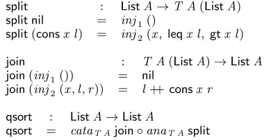
Example 6(Quicksort). Assuming a typeA, and two functions, leq, gt : A → List A → List A, that filter the elements appropriately, we can implement na¨ıve quicksort as:
qsort : ListA→ListA qsort nil = []
qsort(consx l) = qsort(leqx l) ++consx(qsort(gtx l)) We make the recursive structure explicit by using a tree. Thesplit function unfolds the arguments into this tree, and thejoinfunction then flattens it.
split : ListA→TreeA split nil = empty
split(consx l) = node(split(leqx l))x(split(gtx l))
join : TreeA→ListA
join empty = nil
join(nodel x r) = joinl++consx(joinr)
qsort : ListA→ListA qsort = join◦split
We can remove the explicit recursion from these definitions, since splitis a tree anamorphism, andjoinis a tree catamorphism.
split : ListA→T A(ListA) split nil = inj1()
split(consx l) = inj2(x, leqx l, gtx l)
join : T A(ListA)→ListA join(inj1()) = nil
join(inj2(x,l,r)) = l++consx r
qsort : ListA→ListA
qsort = cataT Ajoin◦anaT Asplit
Finally, since we have a composition of a catamorphism and an anamorphism, we can writeqsortas the equivalent hylomorphism.
qsort=hyloT Ajoin split
The only construct that has not yet been considered is feedback. Although the fixpoint combinator Y can be easily defined as a hylomorphism, we take a different approach. Observe that we can unfold the definition ofiteras follows:
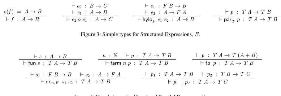
ρ(f) = A→B `f : A→B
`e2 : B→C
`e1 : A→B
`e2◦e1 : A→C
`e1 : F B→B
`e2 : A→F A
`hyloFe1e2 : A→B
[image:5.612.78.532.72.227.2]`p : T A→T B `parTp : T A→T B
Figure 3: Simple types for Structured Expressions,E.
`s : A→B `funs : T A→T B
n : N `p : T A→T B
`farmn p : T A→T B
`p : T A→T(A+B) `fb p : T A→T B `s1 : F B→B `s2 : A→F A
`dcn,F s1s2 : T A→T B
`p1 : T A→T B `p2 : T B→T C
`p1kp2 : T A→T C
Figure 4: Simple types for Structured Parallel Processes,P.
Note that iff,g : A+B→C, the functionfOg : A+B→C can be written as the composition ofidOid : C+C →Cand f +g : A+B→C+C. We use this to rewriteiteras follows:
iter f = (iter fOid)◦f = (idOid)◦(iter f +id)◦f Iff :A→A+B, we define the functor(+B), with the morphism (+ B) f = f +id, which trivially preserves identities and composition. Sinceiter f = (idOid)◦(+B) (iter f)◦f, then:
iter f = hylo(+B)(idOid)f
3.3 Structured Expressions
We have now seen that the denotational semantics of all our parallel constructs can be given in terms of hylomorphisms. This semantic correspondence is not unexpected since it has been used to describe the formal foundations of data-parallel algorithmic skeletons [28]. We take this correspondence one step further by using hylomor-phisms as a unifying structure, and by then exploiting the reason-ing power provided by the fundamental laws of hylomorphisms. In order to define our type-based approach, we will first define a new language,E, that combines two levels,Structured Expressions (S), that enable us to describe a program as a composition of hy-lomorphisms; andStructured Parallel Processes(P), that build on S using nested algorithmic skeletons. A program inE is then ei-ther a structured expressions ∈ Sor a parallel programparTp, wherep∈P. Our revised syntax is shown below. Note that since a p∈Pcan only appear under aparTconstruct, we no longer need to annotate eachfunanddcwith the collectionTof tasks.
e∈E ::= s | parTp
s∈S ::= f | e1 ◦ e2 | hyloF e1e2
p∈P ::= funs|p1kp2|dcn,F s1s2|farmn p|fbp
The denotational semantics of P only changes in the rules that mentione, and by providing a semantics forparT:
JparTpK = mapTSJpK
. . .
SJfuneK = JeK
SJdcn,Fe1e2K = hyloFJe2K Je1K
. . .
The corresponding typing rules are entirely standard (Figures 3–4). Finally, it is convenient to define the “parallelism erasure ofS”,S. Intuitively,Scontains no nested parallelism: for alls∈S,s ∈S if and only ifscontains no occurrences of theparTconstruct. This is equivalent to definings in the erasure of S, S, if it is just a composition of atomic functions and hylomorphisms:
s∈S ::= f | s1 ◦ s2 | hyloFs1s2
The structure-annotated type system given in Section 4 below de-scribes how to introduce parallelism to ans∈Sin a sound way.
3.3.1 Soundness and Completeness.
It is straightforward to show that the type system from Figs. 3– 4 is both sound and completewrtour denotational semantics. Our soundness property is:∀e ∈ E; A,B ∈ Type, ` e : A → B =⇒ (JeK∈ JA→BK). The proof is by structural induction
over the terms inE, using the definitions of`e:Tfrom Figs. 3– 4 andJ.Kabove. The corresponding completeness property is:∀e∈
E; A,B ∈ Type, (JeK∈ JA →BK) =⇒ ` e :A →B. The
proof is also by structural induction over the terms inE, using the definitions of`e:A→Bfrom Figs. 3– 4 andJ.Kabove.
4.
A Type System for Introducing Parallelism
In this section, we present a rigorous way to introduce parallelism without affecting a program’s functional behaviour. We annotate top-level program types with an abstraction of thestructureof the program,σ ∈ Σ. We define the associated type system together with mechanisms for reasoning about these programs using this structure. Intuitively,Σis a “pruned” version ofE that retains in-formation abouthowthe computation is performed, while remov-ing as many details as possible aboutwhatis being computed.Definition 4.1(Families of equivalent programs). We say that an e∈Eis in the family of programs that are functionally equivalent tos ∈S,e ∈ Es,if and only ife E s, for the relationE that is defined later in this section.
Let=extdenote extensional equality:f =ext g⇔ ∀x,f x = g x. Since this is not decidable, we use instead a decidable relationE which implies extensional equality. EachEs is a family of pro-grams indexed by their structure, i.e. for each familyEs, there is a functionφs : Σ →Es that returns ane ∈Eswith the desired
structure. Note that not all structuresσ ∈Σare indices of a fam-ilyEs, soφs is a partial function. Given a structureσ ∈ Σand as ∈ S, we use a superscript,sσ, as notation forφs(σ). We de-fine the structureΣand the relationElater in this section, and the functionφsin Section 5.
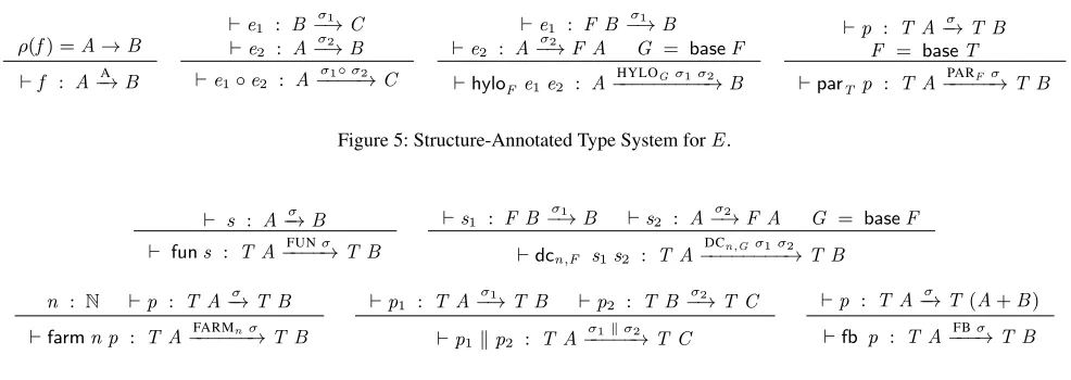
ρ(f) =A→B `f : A−→A B
`e1 : B σ1 −→C `e2 : A
σ2 −→B `e1◦e2 : A
σ1◦σ2 −−−−→C
`e1 : F B σ1 −→B `e2 : A
σ2
−→F A G = baseF `hyloFe1e2 : A
HYLOGσ1σ2 −−−−−−−−−→B
`p : T A−→σ T B F = baseT `parTp : T A
PARFσ
[image:6.612.59.552.73.248.2]−−−−−→T B
Figure 5: Structure-Annotated Type System forE.
` s : A−→σ B ` funs : T A−−−−→FUNσ T B
`s1 : F B σ1
−→B `s2 : A σ2
−→F A G = baseF `dcn,F s1s2 : T A
DCn,Gσ1σ2 −−−−−−−−→T B
n : N `p : T A−→σ T B
`farmn p : T A FARMnσ
−−−−−−→T B
`p1 : T A σ1
−→T B `p2 : T B σ2 −→T C `p1kp2 : T A
σ1kσ2 −−−−−→T C
`p : T A−→σ T(A+B) `fb p : T A−−−→FBσ T B
Figure 6: Structure-Annotated Type System forP.
By typecheckings : A 7−→σ B, the type system guarantees that there is an equivalent program with structureσ,sσ ∈Es. That is, the structured expressionstypechecksif and only if σis an index of the familyEs. The definition ofφs is actually an algorithm for deriving a parallel program from a sequential program and a type-level structure, i.e.φsprovides a mechanism for selecting a parallel program that is equivalent tosand has structureσ, for well-typed programs. We state this formally in the form of our main soundness and completeness properties later in this section.
4.1 The Structure-Annotated Type System
The program structure abstraction,σ∈Σ, is defined below.
σ ∈Σ ::= σs|PARFσp
σs∈Σs ::= A|σ◦σ|HYLOFσ σ
σp∈Σp ::= FUNσs | DCn,Fσsσs
| σpkσp | FARMnσp | FBσp
Figs. 5– 6 define the annotated type system that extends our simple type system from Figs. 3– 4, and that associates expressionse ∈E with structuresσ∈Σ. As before, the global environment,ρ, maps primitive functions to their types. The simple annotated arrow, e : A −→σ B, states thate hasexactlythe structureσ. In order to defineA7−→σ B, we need to extend the type system further with aconvertibility relation.
4.1.1 Convertibility.
We extend our type system with a non-structural rule that captures theconvertibility relation,≡, forΣ.
`e : A−→σ1
B σ1≡σ2
`e : A σ2 7−→B
≡ is defined in terms of the relations≡s∈ Σs×Σs and ≡p∈
Σp×Σp, plus a rule that links theΣsandΣplevels,PAR-EQUIV.
σ1≡sσ2
σ1≡σ2
σ1≡pσ2
PARFσ1≡PARFσ2
PARF (FUNσ)≡MAPFσ (PAR-EQUIV)
The structuresMAPand ITERare defined in Section 5, and
repre-sent the structures of the corresponding hylomorphisms. We de-fine a number of equivalences, starting with≡p. A parallel pipeline
structure (k) is functionally equivalent to a function composition; a task farmFARMcan be introduced for any structure; and
divide-and-conquerDCand feedbackFBcan be derived from hylomorphisms.
FUNσ1kFUNσ2 ≡p FUN(σ2◦σ1) (PIPE-EQUIV) DCn,Fσ1σ2 ≡p FUN(HYLOFσ1σ2) (DC-EQUIV) FARMnσ ≡p σ (FARM-EQUIV) FB(FUNσ) ≡p FUN(ITERσ) (FB-EQUIV) These equivalences, plus reflexivity, symmetry and transitivity, de-fine an equational theory that allows conversion between different parallel forms, as well as conversion between structured expres-sions and parallel forms, as required by our type system. In these equivalences, we implicitly assume the necessary well-formedness constraints: any structure under aFUNorDCmust be inΣs, and the
structure underFARMmust be inΣp. Note that, thanks to the
tran-sitivity of≡, we can use these simple equivalences to derive inter-esting properties of our parallel structures. For example, the asso-ciativity of parallel pipelines does not need to be defined explicitly, since it can be derived from the associativity of composition. We defer the definition of≡sto Section 4.2.
Definition 4.3(Convertibility inE). For all convertibility rules inΣ, there is an equivalent rule inE. We define the equivalence relationE ∈E×E to be the relation≡lifted toE.
An example that illustrates this is that thePIPE-EQUIVrule
corre-sponds to the rule(funs1kfuns2) Ep (fun(s2◦s1)).
Lemma 1. Semantic equivalence. ∀e1,e2 ∈ E, e1 E e2 ⇒
Je1K =ext Je2K
Proof Sketch.Straightforward by induction on the structure of the equivalence relationE, using the denotational semantics ofP, and the laws of hylomorphisms (Section 5).
As a consequence of Lemma 1, theE relation can be used to define the familiesEs. Any extension to≡ and E may expose more opportunities for parallelisation inEs. There remains only the definition of the functionφs. We defer this to Section 5, together with the decision procedure for≡andE.
4.1.2 Soundness and Completeness.
hyloFinF outF = idµF HYLO-REFLEX
hyloF(f ◦η)g = hyloGf (η◦g) ⇐ η : F →G HYLO-SHIFT
(hyloFf h1) ◦ (hyloFh2g) ⇐ h1◦h2=id HYLO-COMPOSE
f1◦(hyloFg1g2)◦f2 = hyloFg
0 1g
0
2 ⇐ f1strict ∧ f1◦g1=g10◦F f1 ∧ g2◦f2=F f2◦g20 HYLO-FUSION
[image:7.612.335.533.182.409.2]hyloFf gstrict ⇐ f,gstrict HYLO-STRICT
Figure 7: Hylomorphism Laws
theorems for convertibility ensure that the type system derives only functionally equivalent parallel structures from structured expres-sions. The proofs of these properties build on a number of details that are introduced in Section 5.
Theorem 1. Soundness of Conversion.
∀s∈S, σ∈Σ, `s:A7−→σ B ⇒ sσ∈Es
Proof Sketch.Sincesσis a synonym forφ
s(σ),sσis inEsifφsis defined forσ. This property follows directly from the definition of
φs(σ)(Def. 5.1) and from Thm 3 in Section 5.
A straightforward consequence of the soundness of the conversion and of Lemma 1 is that if a structured expression typechecks with typeA7−→σ B, then there always exists a functionally equivalente whose structure isσ.
Corollary 1. ∀s∈S, σ∈Σ, `s:A7−→σ B ⇒ ∃e∈E such that e : A−→σ BandJeK=extJsK.
Theorem 2. Completeness of Conversion.
∀s∈S;σ, σ0∈Σ; s : A σ
0
−→B∧sσ∈Es ⇒ `s:A7−→σ B
Proof Sketch.This follows directly from the definition ofφs(σ) (Def. 5.1) and Thm 3 in Sec. 5.
4.2 Functional Equivalence
The proofs of soundness and completeness rely on a decision pro-cedure for≡, as well as on the definition of theφsfunction for the familiesEs. The definition of≡requires a definition of≡s∈Σs×
Σs. Our≡sadapts the well known hylomorphism laws (Fig. 7) [5,
10, 22], using restricted instances of those laws. These restrictions serve two purposes: i) we avoid checkingstrictnessconditions by simply ensuring that all the functions we use are strict; ii) because the equivalences that we can capture are very limited if we assume no knowledge ofatomic functions, due to the side conditions on the rules, we expose extra structure in our programs.
1. We explicitly represent theinF,outFandidfunctions, with the obvious denotational semantics.
2. We explicitly represent the section of a bifunctorFapplied to a structured expressions, asF srather thanF sid. This, plus the strictness assumption, enables us to apply some limited forms ofHYLO-SHIFTandHYLO-FUSION.
3. We explicitly represent M and O (Fig. 1). Although we do not define equivalences for these combinators, we use them to define theITERstructure later.
s∈S ::= f | hprimi |e1 ◦ e2|hyloFe1e2
prim ::= inF|outF|id|e1hopie2|F e
op ::= O| M
σs∈Σs ::= . . . |IN|OUT|ID|σ1hopiσ2|Fσ
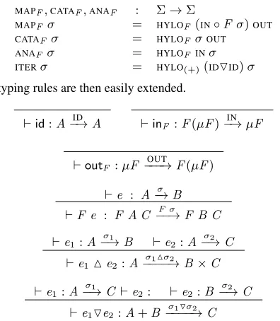
With these structures, we can define the special cases ofHYLOF:
MAPF,CATAF,ANAF : Σ→Σ
MAPFσ = HYLOF(IN◦Fσ)OUT CATAF σ = HYLOFσOUT ANAFσ = HYLOF INσ ITERσ = HYLO(+)(IDOID)σ
The typing rules are then easily extended.
`id:A−→ID A `inF :F(µF)−→IN µF
`outF:µF −−−OUT→F(µF) `e : A−→σ B `F e : F A C−−→Fσ F B C `e1 :A
σ1
−→B `e2:A σ2 −→C `e1Me2:A
σ1Mσ2 −−−−→B×C `e1 :A
σ1
−→C `e2: `e2:B σ2 −→C `e1Oe2:A+B
σ1Oσ2 −−−−→C
Theconvertibility relationis also extended to include some equiv-alences that are derived from the hylomorphism laws:
ID◦σ ≡s σ (ID-LEFT)
σ◦ID ≡s σ (ID-RIGHT)
OUT◦IN ≡s ID (OUT-IN-ID)
IN◦OUT ≡s ID (IN-OUT-ID)
HYLOF IN OUT ≡s ID (HYLO-ID) F(σ1◦σ2) ≡s Fσ1◦Fσ2 (F-COMP)
HYLOF σ1σ2 ≡s CATAF σ1◦ANAFσ2 (HYLO-COMP)
CATAF(σ1◦Fσ2) ≡s CATAFσ1◦MAPFσ2 (CATA-COMP)
ANAF(Fσ1◦σ2) ≡s MAPF σ1◦ANAFσ2 (ANA-COMP)
ANAF(Fσ1◦OUT) ≡s MAPFσ1 (ANA-MAP) We extendE in the expected way with the lifted≡s,Es. The rule
HYLO-COMP is derived from the HYLO-COMPOSE law. The rules
CATA-COMP and ANA-COMP are derived fromHYLO-FUSION. It is easy to see how any strictness condition holds in those rules. Fi-nally, the ruleANA-MAPis derived from theHYLO-SHIFTlaw. It is used only to give a uniform representation of theMAPFstructure.
5.
Determining Functional Equivalence
Recall that for alls ∈S, there is aΣ-indexed familyEs. For all well-typed structured expressions : A 7−→σ B,σis an index of the family defined bys, i.e.sσ ∈E
s. The functionφs : Σ→Es is a partial function whose result is defined for any structureσthat is an index of the familyEs. Given ans : A σ
0
−→ B, both the typechecking algorithm and the functionφsneed to decide whether
ID◦σ s σ (ID-CANCEL-L)
σ◦ID s σ (ID-CANCEL-R)
OUT◦IN s ID (OUT-IN-CANCEL) F(σ1◦σ2) s Fσ1◦Fσ2 (F-SPLIT)
IN◦OUT s ID (IN-OUT-CANCEL)
HYLOFIN OUT s ID (HYLO-CANCEL) FID s ID (F-ID-CANCEL)
ANAF(Fσ1◦OUT) s MAPFσ1 (ANA-MAP)
HYLOFσ1σ2 s CATAFσ1◦ANAFσ2 ⇐ σ16=IN ∧ σ26=OUT (HYLO-SPLIT)
CATAF(σ1◦Fσ2) s CATAFσ1◦MAPFσ2 ⇐ σ16=IN (CATA-SPLIT)
[image:8.612.60.546.77.161.2]ANAF (Fσ1◦σ2) s MAPFσ1◦ANAFσ2 ⇐ σ26=OUT (ANA-SPLIT)
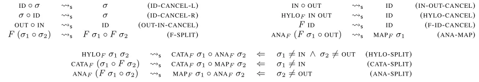
Figure 8: Rewriting system inS
to produce a novel decision procedure for the equality of terms. We consequently use a basic decision procedure, but one that enables interesting parallelisations.
5.1 Reforestation.
We take the standard approach of using term rewriting systems to decide equality inΣ(and henceE). It is well known that if a rewrit-ing system is confluent, then two terms have the same normal form if and only if they are equal with respect to the underlying equa-tional theory. If we define a confluent term rewriting system with ≡as underlying theory, we can use the syntactic equality of nor-malised forms as our decision procedure. We present the rewriting system in two parts. The first part is derived from orienting the rules in≡so that parallelism is erased:
FARMnσp p σp
FUNσ1kFUNσ2 p FUN(σ1◦σ2) DCn,Fσ1σ2 p FUN(HYLOFσ1σ2)
FB(FUNσ1) p FUN(ITERσ1)
PART(FUNσs) p MAPTσs
The first four rules rewrite terms inΣpto terms inΣp, and the last
rule rewrites terms inΣto terms inΣ. We defineΣsin an analogous
way toS, anderaseas any normalisation procedure for a rewriting system p:
erase : Σ→Σs
eraseσ = σ0,s.t.σ *
pσ
0 ∧
@σ00s.t.σ00 pσ00
Lemma 2. The rewriting system pis confluent.
Proof Sketch.The rewriting system is terminating, since the num-ber of redexes is precisely the numnum-ber of parallel structures (includ-ingPART), which is reduced following each rewriting step. It is also easy to show that any critical pairs arising from these rules have the same normal form. For example, a farm of a pipeline reduces to the same expression regardless of which structure is erased first. By Newman’s lemma [1] we can conclude that pis confluent.
Since pis confluent, we know that the result oferaseis unique.
Recall that all the results that are derived from the equational theory≡can be lifted toE. This implies that there is aneraseE : E → S procedure that is equivalent to erasedefined with the rewritings lifted toE. The second step is the normalisation ofσ∈ Σs. We once again use a confluent rewriting system derived from
≡s, and define it modulo associativity of the composition◦. The
direction of the rewriting is chosen so a “reforestation” rewriting is performed. Hylomorphisms are first split into catamorphisms and anamorphisms, which are then themselves split into compositions of maps, catamorphisms and anamorphisms. We omit some trivial cases, e.g.F σ◦F σ−1
ID, and prioritise the rules that deal
with ID to simplify the confluence of the rewriting system. We
only consider the inversesINand OUT,F INandF OUT, etc. For
uniformity reasons,ANA-MAPis applied to the anamorphisms that perform a map computation.
Lemma 3. The term rewriting system sis confluent.
Proof Sketch.The rewriting system is terminating, since the pre-conditions of the rules ensure that no cycles are introduced. The rewriting system is also locally confluent. It is trivial to observe that any critical pair arising from theIDrules have the same
nor-mal form. The critical pairs arising from rules MAP-SPLIT and CATA/ANA-SPLITcan be reduced to the same normal form, by
apply-ingF-SPLITandCATA/ANA-SPLITand/orANA-MAPin a different or-der. For example, we can rewrite anyCATAF(σ1◦F(σ2◦σ3)) *s
CATAF σ1◦MAPF σ2◦MAPFσ3. Any problems that appear from the critical pairs of theIDrules and theSPLITrules can be solved
by forcing theIDrules to be applied first, and working modulo
associativity. As before, Newman’s lemma completes the proof.
Finally, we define the normalisation procedures forΣsandΣ.
normsσ = σ0,s.t.σ *sσ0 ∧ @σ00s.t.σ0 sσ00
norm = norms◦erase
We use a subscript,normE, to denote this normalisation procedure lifted toE. Given that the underlying equational theory of the term rewriting system isE, we know that:∀e1,e2 ∈E,(normE e1 =
normEe2)⇔(e1!*e2)⇔(e1Ee2).
Theorem 3(norm defines a decision procedure for≡). For all
σ1, σ2∈Σ,σ1≡σ2if and only ifnormσ1=normσ2.
Proof Sketch.From the properties of p, we derive that it is always
true thatσi ≡eraseσi. Since sis confluent, by the properties
of term rewriting systems, we know thateraseσ1 ≡ eraseσ2 if and only ifnorms(erase(σ1)) =norms(erase(σ2)). We finish the
proof by combining these two facts using the transitivity of≡with the definition ofnorm.
The fact that we can lift the results fromΣtoE implies that we can use this rewriting system not only to reason about program equivalences, but also to define an algorithm toderivea parallel program from somes ∈Sand a type-level parallel structure. We sketch this algorithm as the definition ofφs.
Definition 5.1(φs). Lets∈S,σ1∈Σs, such that`s:A
σ1 −→B, andσ2∈Σ. We defineφs(σ2)as follows:
Letσi0=normσi. Ifσ 0 1=σ
0 2, then:
1. Reverse the rewriting steps fromσ2toσ20:σ20 *σ2.
2. Obtain the proof ofσ1≡σ2by usingσ1 *σ01and (1).
3. Obtain the rewriting stepsσ1 *σ2
from (2). 4. Lift the rewriting steps toE, and apply them tos:s *
EQ ∆ ={{}}
σ∼σ⇒∆ META
r 1
∆ ={{m∼σ}}
m∼σ⇒∆ MAP1
σ1∼σ01⇒∆1
Fσ1∼Fσ01⇒∆1
MAPr2
σ1◦σ2∼F m2◦F m3⇒∆2
∆1={{m1∼m2◦m3}} σ1◦σ2∼F m1⇒∆1⊗∆2
COMP1
σ1∼σ01⇒∆1 σ2∼σ02⇒∆2 σ1◦σ2∼σ01◦σ02⇒∆1⊗∆2
COMPr2
σ1◦σ2∼σ01⇒∆11 σ3∼σ20 ⇒∆12 σ2◦σ3∼σ02⇒∆22 σ1∼σ10 ⇒∆21 σ1◦σ2◦σ3∼σ10◦σ20 ⇒∆11⊗∆12∪∆21⊗∆22
OP σ1∼σ
0
1⇒∆1 σ2∼σ20 ⇒∆2 σ1hopiσ2∼σ01hopiσ
0
2⇒∆1⊗∆2
HYLO1
σ1∼σ01⇒∆1 σ2 ∼σ02⇒∆2
HYLOFσ1σ2∼HYLOFσ01σ 0
2⇒∆1⊗∆2
HYLOr2 σ1◦σ2 ∼ HYLOFm1OUT◦HYLOF INm2⇒∆1 σ1◦σ2 ∼ HYLOFm1OUT⇒∆2 σ1◦σ2 ∼ HYLOFINm2⇒∆3
σ1◦σ2 ∼ HYLOFm1m2⇒∆1∪ {{m2∼OUT}} ⊗∆2∪ {{m1∼IN}} ⊗∆3
HYLOr3
σ1◦σ2 ∼HYLOF(IN◦F m2)OUT◦HYLOFINm3⇒∆1 σ1◦σ2 ∼HYLOF (IN◦F m2)OUT⇒∆2 ∆ ={{m1∼F m2◦m3}}
σ1◦σ2 ∼ HYLOFINm1⇒∆⊗∆1∪∆⊗ {{m3∼OUT}} ⊗∆2
HYLOr4 σ1◦σ2 ∼
HYLOFm2OUT◦HYLOF(IN◦F m3)OUT⇒∆
σ1◦σ2 ∼ HYLOFm1OUT⇒ {{m1∼m2◦F m3}} ⊗∆
HYLOr5 σ1◦σ2 ∼HYLOFm1OUT◦HYLOF INσ3⇒∆1 σ1◦σ2∼norm(HYLOFINσ3)⇒∆2 σ36=OUT
σ1◦σ2∼HYLOFm1σ3⇒∆1∪ {{m1∼IN}} ⊗∆2
HYLOr6 σ1◦σ2 ∼HYLOFσ3OUT◦HYLOFINm1⇒∆1 σ1◦σ2∼norm(HYLOFσ3OUT)⇒∆2 σ36=IN
σ1◦σ2∼HYLOFσ3m1⇒∆1∪ {{m1∼OUT}} ⊗∆2
HYLOr7
σ1◦σ2∼HYLOF (IN◦F m2)OUT◦HYLOF(IN◦F m3)OUT⇒∆
[image:9.612.64.549.82.387.2]σ1◦σ2∼HYLOF(IN◦F m1)OUT⇒ {{m1∼m2◦m3}} ⊗∆
Figure 9: Unification Rules.
Since the typechecking algorithm for our type system needs to decideσ1≡σ2(e.g. using Thm. 3), steps(1)to(2)can be omitted if we know that` s : A σ2
7−→ B (recall the proof of Thm. 1). Conversely, if there is somes`A−→σ1 B, andsσ2 ∈Es, we know that there is a proofσ1 ≡σ2(step (2) in Def. 5.1), and therefore s`A7−→σ2 B(recall the proof of Thm. 2).
5.2 Structure Unification.
The structure-annotated types that we have presented so far require the specification of a full structureσ∈Σ. However, it is sometimes sufficient, or desirable, to specify only the relevant parts of this structure. We allow this by introducingstructure metavariablesin Σ. Selecting suitable substitutions for these metavariables can be automated in different ways, as we will see later in this section. Given a set of metavariables, M, we extend the syntax ofΣas follows:
m∈ M
σs∈Σs ::= . . . |m
σ ∈Σ ::= . . .|m
σp∈Σp ::= . . .|m
The underscore character denotes a fresh metavariable, e.g. given a fresh metavariablem,FARMn is equivalent toFARMnm.
Definition 5.2(Substitution Environments). A substitution envi-ronment δ is a mapping of metavariables to structures,{m1 ∼ σ1,m2∼σ2, . . .}. We use∆to denote sets of environmentsδ.
The two basic operations with substitution environments are the applicationand theextension. We apply a substitution environment
δto a structureσ, denoted byδσ, by replacing all metavariables as defined byδ. The extension ofδ1withδ2,δ1δ2, is defined in the
expected way. If both substitution environments introduce a cycle or conflicting metavariables, the operation fails. Finally, for sets of substitution environments, we define the set of extensions:
∆1⊗∆2 = {δ1δ2|δ1∈∆1∧δ2∈∆2}
Lemma 4. For all substitutionsδ, for allσ ∈ Σ, normδσ ≡
δ(normσ).
Proof Sketch.It is obvious that if σ1 ≡ σ2, then δσ1 ≡ δσ2, sinceδwill apply the same substitution in bothσ1 andσ2. Since
σ≡normσ, we conclude using the reflexivity of≡.
Note that we can no longer use the relation≡in our typechecking rules, since it does not handle metavariables. Instead, we define the relation∼=, and define a decision procedure for it.
Definition 5.3(Equivalence of the Unified Forms). We say that
σ1∼=σ2if there is at least a substitutionδthat makesδσ1≡δσ2.
σ1∼=σ2=. ∃δ, δσ1≡δσ2
The type rule for equivalence changes to use the new relation:
`e : A−→σ1 B σ1∼=σ2
`e : A7−→σ2 B
1. Anyerasestep on a structure with meta-variables always suc-ceeds by simply adding new meta-variables and a substitution environmentδfor those metavariables, e.g.
m1km2 FUN(m20◦m10)
δ={m1∼FUNm10,m2∼FUNm20}.
2. The constraints of the rules used by thenormS procedure are modified so that they are never satisfied by metavariables, e.g.
HYLOFσ1σ2 s CATAFσ1◦ANAFσ2 (HYLO-SPLIT) ⇐ σ1 6=IN ∧ σ26=OUT ∧ σ16∈ M ∧ σ26∈ M
Although condition 2 is not necessary, it simplifies the unification of structures whereσ1orσ2can be unified toINorOUT.
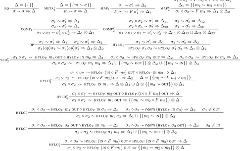
Unification Rules. Since unifying two structures may lead to different, but valid unifying substitutions, the unification rules yield the set of all possible unifying substitutions, ∆. Disambiguating such situations can be done using cost models, or some other procedure. The rules for unification (Fig. 9) define a unification modulo associativity (ruleCOMP2). Each rule with superscriptrhas
a symmetric versionl. A statementσ1 ∼ σ2 ⇒ ∆means that structureσ1 unifies with structureσ2, under a non-empty set of substitutions,∆6=∅. Whenever two structures do not correspond
to the same syntactic structure, the unification rules make any valid assumption about the metavariables that would allow further rewritings to take place.
Theorem 4(Soundness of the Unification). For allσ1, σ2∈Σ,
σ1∼σ2⇒∆ =⇒∆6=∅∧ ∀δ∈∆, δσ1≡δσ2
Theorem 5(Completeness of the Unification). For allσ1, σ2∈Σ, and substitutionδ,
δσ1 ≡δσ2=⇒ ∃∆s.t.∆6=∅∧σ1∼σ2⇒∆
The proofs of those theorems are standard proofs by induction on the derivations of∼and≡, and by case analysis on the metavari-ables.
Corollary 2. ∼=:σ1∼=σ2 ⇔ normσ1∼normσ2⇒∆, i.e. the unification algorithm can be used as a decision procedure for∼=. Proof Sketch.For the proof of the⇒case, we know that there is at least aδsuch thatδσ1 ≡ δσ2. From the properties of≡, we know thatnormδσ1=normδσ2. Using Lemma 4, we derive that
δ(normσ1)≡δ(normσ2). The completeness of the unification allows us to conclude thatnormσ1∼normσ2⇒∆.
The proof of ⇐ follows from the soundness of the unification algorithm. We know that norm σ1 ∼ norm σ2 ⇒ ∆implies that ∆is non-empty, and that for allδ ∈ ∆, δ (norm σ1) ≡
δ(normσ2). We conclude by selecting anyδ from∆, and then using Lemma 4.
Using metavariables in structures has some implications. Given a s ` A −→σ1
B, and a structure σ2 containing one or more metavariables,σ2can no longer be used as an index for a family Es. Since there may be alternative, but valid substitutions for the metavariables, it follows thatsσ2 ⊆Es. Given a unificationσ1 ∼
σ2 ⇒ ∆, we need to apply a δ ∈ ∆to σ2 in order to use it as an index, sδσ2 ∈ Es. This implies that there are many ways to use our approach. On one hand, fixing this σ2 to be a closed structure without any metavariables, or one that unifies withσ1 with a unique substitution, provides a way to manually parallelise a program. On the other hand, ifσ2 is defined to be a metavariable, then a fully automated method for selecting a parallel structure would be needed. In between, there are a wide range of semi-automatedpossibilities that can be used to reason about the introduction of parallelism to a program. The automated selection mechanism for a δ ∈ ∆ can easily be extended with further
parallelisation opportunities. Furthermore, it can be parameterised by architecture-specific details, so that compiling a program for different architectures leads to alternative parallelisations. This is, however, beyond the scope of this paper.
Compositionality and Higher-Order Structured-Arrows. We finish this section with a discussion of the compositionality of our approach. Most of this paper deals with the typing rule for structure-annotated arrows. Extending our work for a language with definitions and with a limited-form of higher-order structured arrows can be done using the unification rules from Fig. 9.
Ap-plying somee : A σ
0 1
7−→ B to af : A 7−→σ1 B → C 7−→σ2 D typechecks only ifσ1 ∼ σ10 ⇒ ∆, and the type of this would
be annotated with a structure resulting from applying anyδ ∈∆, f e:C 7−−→δσ2
D. One advantage of this is to easily allow the spec-ification of new structures that can be later used in our programs. The corresponding erasure rules would then be derived automati-cally from such a specification. We would need, however, to verify a back-end for such a language in order to ensure that the oper-ational semantics of the new structures are sound with respect to the specification. Although we do not explain this idea in detail in this paper, we will use a small example of a defined structure in Section 6.3.
Although it seems entirely feasible to support full higher-order structured arrows, there is the question of whether this is desirable: what would types such asA 7−→σ B 7−→σ0 C or (A 7−→σ B) 7−→σ0 C mean? Intuitively, the first would be a parallel process with structureσthat produces a parallel process with structureσ0, and the second would be a parallel process with structureσ0that takes a parallel process with structureσas input, and produces an output of type C. In contrast to using functions with a type such as X σ1
7−→ Y → A σ2
7−→ B, we have so far not seen the benefits of full higher-order functions in our examples, although this is an idea that may be worth exploring in future work.
6.
Examples
Our first two examples revisitimage mergefrom Section 1, and quicksortfrom Section 3. In both cases, we show how the type sys-tem calculates the convertibility of the structured expression to a functionally equivalent parallel process, and how the convertibility proof allows the structured expression to be rewritten to the de-sired parallel process. The final two examples show how to use types to parallelise different algorithms, described as structured ex-pressions. These examples show how to easily introduce parallel structure to these algorithms using our type system.
6.1 Image Merge
Recall thatimage mergebasically composes two functions:mark andmerge. It can be directly parallelised using different combina-tions of farms and pipelines.
IM1(n,m) = PARL(FARMn(FUN A)k FARMm(FUN A))
imageMerge : List(Img×Img) 7−−−−−−→IM1(n,m) List(Img×Img) imageMerge = mapList(merge ◦ mark)
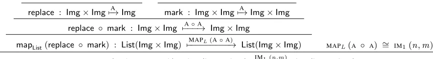
First, we use our annotated typing rules to produce a derivation tree with the structure of the expression (Fig. 10). The key part is the convertibility proof, thatMAPL(A ◦A) ∼= IM1(n,m). We use the
decision procedure defined in Section 4 to decide the equivalence of both structures. Theerasestep is applied as follows:
replace : Img×Img7−→A Img mark : Img×Img7−→A Img×Img replace ◦ mark : Img×Img 7−−−→A◦A Img×Img
mapList(replace ◦ mark) : List(Img×Img)
MAPL(A◦A)
7−−−−−−−−−→ List(Img×Img) MAPL(A ◦ A) ∼= IM1(n,m)
mapList(replace ◦ mark) : List(Img×Img)
IM1(n,m)
[image:11.612.81.524.77.138.2]7−−−−−−→ List(Img×Img)
Figure 10: Typing Derivation Tree for Image Merge
The final step involves applying the decision procedure for equality ofS. Since the expressions are identical, this is a trivial step. We can now apply this equivalence to the original expression:
mapList(merge ◦ mark) *
parList(farmn(fun mark)kfarmm(fun merge)) We now show an example of unification. We define IM2 n =
PARL( k FARMn ). First, we instantiate the structure with fresh metavariablesm1 andm2. Then, we normalise the structure. We
start by applying theeraserewriting system:
MAPL(m20 ◦m 0
1) δ={m1∼FUNm10, m2∼FUNm20}
We then apply the normalisation inΣs, and the unification rules:
MAPLA◦MAPLA∼MAPLm20◦MAPLm10 ⇒ {{m 0 1∼A,m
0 2∼A}}
The final step is to calculate the extension of the environmentδ, and the set of environments that are obtained from the unification:
∆ ={δ} ⊗ {{m0
1∼A,m20 ∼A}}=
{{m1∼FUNm1,0 m2∼FUNm20,m10 ∼A,m20 ∼A}}
Applying the substitution environment in ∆ to the IM2(n), we
obtain the structurePARL(FUN AkFARMn(FUN A)).
Finally, we briefly discuss how to extend the environment fur-ther using a proceduremin cost. First,minattempts further rewrit-ings tom1andm2. To ensure termination, the process stops
when-ever the only option is to introduce a task farm to an existing task farm structure.
δ1={m1 ∼ FARMn1(FUN A), m2 ∼ FARMn2(FUN A)}
δ2={m1 ∼ FUN A, m2 ∼ FARMn2(FUN A)}
δ3={m1 ∼ FARMn1(FUN A), m2 ∼ FUN A}
δ4={m1 ∼ FUN A, m2 ∼ FUN A}
We will show how to select one of those structures using a simple example cost model. In future work, we will consider how to extend and formalise this cost model. A cost model provides size functions|σ|over structures, similar to the idea ofsized types[17]. We assume that all atomic functions are annotated with their cost models,Ac. The cost of a structure is a function that receives a size, sz, and returns an estimation of its run-time in milliseconds.
In our example, we assume thatsz = [d]1000. This represents the size of 1000 pairs of images ofddimensions. Arithmetic op-erations onsz are applied to the superscript. The size function of the first stage|Ac1|is the identity, since we are not modifying the images. The parameters for the number of farm workers are fixed to be those with the least cost, given some maximum number of avail-able cores. In this example, we assume that a maximum of 24 cores are available. Forδ1, we determine thatn1= 9,n= 3andn2= 5.
The values of the costs on those sizes, and the overheads of farms and pipelines (κ1 and κ2) are given below. In the following ex-amples, we omit these numbers and just provide the estimation for a 24-core architecture with similar overheads for farms, pipelines,
divide-and-conquer and feedback.
c1[(2048×2048,2048×2048)]n = n×25.11ms
c2[(2048×2048,2048×2048)]n = n×45.21ms κ1(9) = 29.66ms κ1(3×5) = 60.93ms
κ2(9,3×5) = 114.4ms
cost(δ1IM2(n))sz
= max{c1(
sz n1
) +κ1(n1),c2(
|Ac1|(sz) n×n2
) +κ1(n×n2)}
+ κ2(n1,n×n2) = 3145.69ms
cost(δ2IM2(n))sz = 25123.81ms
cost(δ3IM2(n))sz = 3189.60ms
cost(δ4IM2(n))sz = 25123.81ms
The structure that results from applyingδ1 is the least cost one,
δ1(IM2(3)), withn1= 9andn2= 5.
6.2 Quicksort
We will now revisitquicksortand show how it can exploit a divide-and-conquer parallel structure.
qsorts : List(ListA)→List(ListA) qsorts = mapList(hyloF Amerge div)
In order to introduce a divide-and-conquer parallel structure, the type system needs to decide:
MAPL(HYLOFA A)∼=PARL(DCn,FA A)
This can be achieved using a simple parallelism erasure. Consider now a slightly more complex structure:
MAPL(HYLOFA A) ∼= PARL(FARMn k )
Letm1,m2be two fresh metavariables. The parallelism erasure of
the right hand side returns the following structure and substitution:
PARL(FARMn m2km1) * MAPL(m10◦m 0 2) δ={m1 ∼ FUNm10,m2∼FUNm20}
The normalisation procedure continues by normalising the left and right hand sides of the equivalence following a parallelism erasure. The left hand side is normalised by applyingHYLO-SPLIT,F-SPLIT
andCATA-SPLIT:
MAPL(HYLOFA A) *MAPL(CATAFA) ◦ MAPL(ANAF A) The right hand side of the equivalence is normalised by applying
F-SPLITandCATA-SPLIT:
MAPL(m10 ◦m20) *MAPLm10 ◦MAPLm20
The decision procedure finishes by unifying both structures, and extending the substitutionδwith all possible unifications.
MAPL(CATAFA) ◦ MAPL(ANAF A)∼MAPLm10◦MAPLm20
⇒∆1={m10 ∼CATAFA,m20 ∼ANAF A}
Again, by applying the only substitution inδ0 ∈ ∆, we select the final structure:
PARL(FARMn(FUN(ANAFA))kFUN(CATAFA))
The full proof of equivalence (∼=) allows us to rewrite quicksort to our desired parallel structure:
mapList(hyloF Amerge div)
*
parList(farmn(fun(anaF Adiv)) k fun(cataF Amerge))
We can use our cost model again, where κ3 is the overhead of a divide-and-conquer structure. In this example, we set the size parameter of our cost model to 1000 lists of 3,000,000 elements, and use the following structure:
qsorts : List(ListA)7−−−−−→min cost List(ListA) cost(PARL(DCn,FAc1Ac2))sz
= max{max
1≤i≤n{c2(|Ac2| i
sz)
,cost(HYLOF Ac1Ac2) (|Ac2| n
sz)
, max
1≤i≤n{c1(|Ac1|
i|
Ac2| n
sz)}} + κ3(n) = 42602.72ms
cost(PARL(FARMn(FUN(ANALAc2))k(FUN(CATALAc1))))sz = 27846.13ms
cost(PARL(FARMn(FUN(HYLOFAc1Ac2))))sz = 32179.77ms
. . .
Since the most expensive part of the quicksort is the divide, and flattening a tree is linear, the cost of adding a farm to the divide part is less than using a divide-and-conquer skeleton for this example.
6.3 N-Body Simulation
N-Body simulations are widely used in astrophysics. They com-prise a simulation of a dynamic system of particles, usually under the influence of physical forces. The Barnes-Hut simulation recur-sively divides thenbodies storing them in aOctree, or a8-ary tree. Each node in the tree represents a region of the space, where the topmost node represents the whole space and the eight children the eight octants of the space. The leaves of the tree contain the bod-ies. Then, the cumulative mass and center of mass of each region of the space are calculated. Finally, the algorithm calculates the net force on each particular body by traversing the tree, and updates its velocity and position. This process is repeated for a number of iterations. We will here abstract most of the concrete, well known details of the algorithm, and present its high-level structure, using the following types and functions:
C = Q×Q
F A B = A + C×B8
G A = FBody
Octree = µG
insert : Body×Octree→Octree
Since this algorithm also involves iterating for a fixed number of steps, we define iteration as a hylomorphism. We assume that the combinator+(Fig. 1) is also defined inΣs. Additionally, we
assume a primitive combinator, that tests a predicate on a value, (·?) : (A→Bool)→A→A+A.
LOOP : Σ→Σ
LOOPσ = HYLO(+)(IDOσ) ((A+ (AM(A◦A)))◦(A◦A?))
loopA : (A7−→m A)→A×N7−−−−−→LOOPm A
loopAs = hylo(A+)(idOs)
((π1+ (π1M((−1)◦π2)))◦((== 0)◦π2)?)
This example uses some additional functions:calcMassannotates each node with the total mass and centre of mass;distdistributes the octree to all the bodies, so that each can independently calculate its forces and update the velocity and position;calcForcecalculates the force of one body; andmoveupdates the velocity and position of the body.
calcMass : GOctree→GOctree dist : Octree×List Body
→L(Octree×Body) (Octree×List Body) The algorithm is:
nbody : List Body×N7−−−−−→LOOPσ List Body
nbody = loop(anaL(L(move◦calcForce)◦dist)
◦((cataG(inG◦calcMass)◦cataLinsert)Mid)) Since the LOOP defines a fixed structure, we do not allow any rewriting that changes this structure. However, note that our type system still enables some interesting rewritings. In particular, the structure of the loop body is:
σ=ANAL(L(A◦A)◦A)◦(CATAG(IN◦A)◦CATALA)MID
The normalised structure reveals more possibilities for introducing parallelism:
σ=MAPLA◦MAPLA◦ANALA◦(CATAG(IN◦A)◦CATALA)MID
After normalisation, this structure is equivalent to:
σ=PARL(FUN(A◦A))◦
The structure makes it clear that there are many possibilities for parallelism using farms and pipelines. As before, parallelism can be introduced semi-automatically using a cost model. For example, setting the input size to 20,000 bodies:
σ =PARL(FARMn k )◦
σ0=PARL(min cost( k ))◦
cost(FUN Ac1kFUN Ac2)sz = 310525.67ms
cost(FARM6(FUN Ac1)k(FUN Ac2))sz = 55755.43ms cost(FUN Ac1kFARM1(FUN Ac2))sz = 310525.67ms cost(FARM20(FUN Ac1)kFARM4(FUN Ac2))sz = 15730.46ms
6.4 Iterative Convolution
Image convolution is also widely used in image processing applica-tions. We assume the typeImgof images, the typeKernof kernels, the functorF A B = A+B×B×B×B, and the follow-ing functions. Thesplitfunction splits an image into 4 sub-images with overlapping borders, as required for the kernel. Thecombine function concatenates the sub-images in the corresponding posi-tions. Thekernfunction applies a kernel to an image. Finally, the finishedfunction tests whether an image has the desired properties, in which case the computation terminates. We can represent image convolution on a list of input images as follows:
conv : Kern→(List Img7−→σ List Img) convk =
The structure of conv is equivalent to a feedback loop, which exposes many opportunities for parallelism. Again, we assume a suitable cost model, and the estimations are given for 1000 images, of size 2048×2048.
σ = PARL(FB(DCn,L,F(A◦F A)Ak ))
= PARL(FB(FARMn k k )) = min cost(PARL(FB( k ))) = . . .
cost(PARL(FB(Ac1kAc2)))sz = P
1≤i,|Ac1kAc2|isz>0
cost(Ac1kAc2) (|Ac1kAc2|
i
sz)
= 20923.02ms
cost(PARL(FB(FARM4(FUN Ac1)k(FUN Ac2))))sz = 6649.55ms
cost(PARL(FB(FUN Ac1kFARM1(FUN Ac2))))sz = 20923.02ms
cost(PARL(FB(FARM14(FUN Ac1)kFARM4(FUN Ac2))))sz = 2694.30ms
. . .
Collectively, our examples have demonstrated the use of our tech-niques for all the parallel structures we have considered, showing that we can easily and automatically introduce parallelism accord-ing to some required structure, while maintainaccord-ing the functional equivalence with the original form.
7.
Related Work
There have been some previous treatments of parallelism using types, but these deal only with sizes and productivity. One line of work is usingsized types[17] to internalise a notion of sizes of streaming data into a type system. This has been extended to a small number of skeletons in the Eden language [27]. While types were useful to prove the termination and productivity of Eden skeletons, our own work focuses on the different, but important, properties of semantic equivalence and cost. The expressive power of hylo-morphisms for parallel programming was first explored by Fischer and Gorlatch [4], who showed that a programming language based on catamorphisms and anamorphisms isTuring-universal. The idea of using hylomorphisms for parallel programming also appears in Morihata’s work [24]. Morihata explores a theory for developing parallelisation theorems based on thethird homomorphism theorem andshortcut fusion, and generalises it to hylomorphisms. In con-trast, our work directly exploits the properties of hylomorphisms, in order to choose a suitable parallel skeleton implementation for hylomorphisms. Both lines of work are therefore orthogonal, and we can potentially benefit from Morihata’s results.
Deriving parallel implementations from small, simple specifi-cations has been widely studied. The third homomorphism theo-rem, list homomorphisms, and the Bird-Meertens Formalism are amongst the many techniques that have been explored [12, 15, 16, 18, 21, 23, 25, 29–31]. The third homomorphism theorem states that if a function can be written both as a left fold and a right fold, then it can also be evaluated in a divide-and-conquer manner [9]. This theorem has been widely used for parallelism [2, 6, 8, 11, 19, 24, 26]. The majority of this work enables suitable automation and derivation of efficient parallel implementations. Our work differs in that we allow part of the parallel structure to be chosen in a semi-automated way. This adds flexibility, enabling a parallel im-plementation to be changed quickly and easily by changing only a single type annotation. One possible extension of our work is to include some automatic transformations derived from the third homomorphism theorem. By parameterising our type system over some cost function on parallel structures, we smoothly integrate the introduction of parallelism with the ability to reason about the
run-time behaviour of the parallel program. Skillicorn and Cai [32] have previously shown the utility of such an integration of a cost cal-culus with derivational software development, illustrating the ap-proach for the Bird-Meertens theory of lists. We take this apap-proach one step further by using a more general equational theory based on hylomorphisms. Moreover, our type-based approach introduces new benefits, by providing a mechanism for specifying new paral-lel structures whose denotational semantics can be described as a composition of hylomorphisms.
Finally, in a practical setting, Steuwer et al [33] generate high-performance OpenCL code from a high-level specification by ap-plying a simple set of rewrite rules, and using Monte-Carlo search to traverse the corresponding search space to find an implementa-tion. Our semi-automated approach provides a way to narrow down this search space, while using cost models to automate the rest. Our approach is in a sense more general, since we allow our parallel structures to be easily extended. However, we could benefit from exploiting their work in GPU-specific rewriting rules and skeletons.
8.
Conclusions
This paper has introduced a new type-based approach for repre-senting and reasoning about the structure of parallel programs rep-resented as algorithmic skeletons,the first ever treatment of par-allelism at the type levelthat combines reasoning about program equivalences and cost. Crucially, our type system is capable of rea-soning about both the functional and the non-functional properties of a parallel program. Given a cost model and the underlying equa-tional theory, we have shown how we can take raequa-tional choices at the type level between alternative parallel implementations by appropriately instantiating and transforming high-level parallelism abstractions. This avoids the usual static analysis approach that sep-arates analysis from program. In particular, all transformations are performed internally by the type checker and we ensure the preser-vation of the underlying functional behavioursimply by construc-tion. It also opens the door to further safe type-level program ma-nipulations, for example. A key aspect of our approach is the use ofhylomorphisms, combinations ofcatamorphisms and anamor-phisms(orfold/unfold operations), as a single, unifying parallel structure. In this paper we have used hylomorphisms to capture many common patterns of parallelism that are found in the litera-ture, includinginter aliatask farms, pipelines, divide-and-conquer and dynamic feedback. As we have shown in our examples, this sin-gle construct is surprisingly powerful, providing a system of canon-ical representations that is easy to understand and to transform.
A number of obvious extensions can be made to this work. Firstly, there are a few forms of parallel pattern that we have not yet considered:map (reduce)andfoldare clearly instances of hy-lomorphisms, butstenciland bulk synchronous parallelpatterns, for example, may require deeper thought. Secondly, more sophis-ticated and accurate cost models are both possible and desirable, including ones that consider e.g. the sizes of data structures. The model we have shown here is, however, more precise and realistic than e.g. typical PRAM models that are widely used in parallelism theory. Thirdly and finally, we have only shown a static analysis here. However, type-based approaches can freely admit dynamic analyses as well. We intend to explore this in future in order to obtain even more general and flexible analyses.
Acknowledgements
This work has been partially supported by the EU H2020 grant “RePhrase: Refactoring Parallel Heterogeneous Resource-Aware Applications - a Software Engineering Approach” (code 644235), and by EPSRC grant EP/M027317/1 “C3: Scalable & Verified
References
[1] F. Baader and T. Nipkow. Term Rewriting and All That. Cambridge
University Press, 1998.
[2] Y.-Y. Chi and S.-C. Mu. Constructing List Homomorphisms from
Proofs. InProc. APLIAS ’11: Asian Symposium on Programming
Languages & Systems, pages 74–88. 2011.
[3] M. I. Cole.Algorithmic Skeletons: Structured Management of Parallel
Computation. Pitman, London, 1989.
[4] J. Fischer and S. Gorlatch. Turing Universality of Recursive Patterns
for Parallel Programming. Parallel Processing Letters, 12(02):229–
246, 2002.
[5] M. M. Fokkinga and E. Meijer. Program Calculation Properties of Continuous Algebras. Technical Report, CWI, 1991.
[6] A. Geser and S. Gorlatch. Parallelizing Functional Programs by
Generalization. Journal of Functional Programming (JFP), 9(06):
649–673, 1999.
[7] N. Ghani. βη-Equality for Coproducts. InProc. International Conf.
on Typed Lambda Calculi and Applications, pages 171–185. 1995.
[8] J. Gibbons. Computing Downwards Accumulations on Trees Quickly.
Theoretical Computer Science, 169(1):67–80, 1996.
[9] J. Gibbons. The Third Homomorphism Theorem. Journal of
Func-tional Programming (JFP), 6(4):657–665, 1996.
[10] J. Gibbons. Calculating Functional Programs. InAlgebraic and
Coalgebraic Methods in the Mathematics of Program Construction, pages 151–203. 2002.
[11] S. Gorlatch. Extracting and Implementing List Homomorphisms in
Parallel Program Development. Science of Computer Programming,
33(1):1 – 27, 1999.
[12] S. Gorlatch and C. Lengauer. Parallelization of Divide-and-Conquer
in the Bird-Meertens Formalism.Formal Aspects of Computing, 7(6):
663–682, 1995.
[13] T. Hardin. Confluence Results for the Pure Strong Categorical Logic CCL.λ-calculi as Subsystems of CCL.Theoretical Computer Science, 65(3):291–342, 1989.
[14] Y. Hayashi and M. Cole. Static Performance Prediction of Skeletal
Parallel Programs. Parallel Algorithms and Applications, 17(1):59–
84, 2002.
[15] Z. Hu, H. Iwasaki, and M. Takechi. Formal Derivation of Efficient
Parallel Programs by Construction of List Homomorphisms. ACM
Transactions on Programming Languages and Systems (TOPLAS), 19 (3):444–461, 1997.
[16] Z. Hu, M. Takeichi, and W.-N. Chin. Parallelization in Calculational
Forms. InProc. POPL ’98: 25th ACM Symposium on Principles of
Programming Languages, pages 316–328, 1998.
[17] J. Hughes, L. Pareto, and A. Sabry. Proving the Correctness of
Reactive Systems Using Sized Types. InProc. POPL ’96: 23rd ACM
Symposium on Principles of Programming Languages, pages 410– 423, 1996.
[18] G. Keller and M. Chakravarty. Flattening Trees. InProc. Euro-Par
’98: European Conference on Parallelism, pages 709–719. 1998.
[19] Y. Liu, Z. Hu, and K. Matsuzaki. Towards Systematic Parallel
Pro-gramming over Mapreduce. InProc. Euro-Par 2011: European
Con-ference on Parallelism, pages 39–50. 2011.
[20] O. Lobachev and R. Loogen. Estimating Parallel Performance, a
Skeleton-Based Approach. InProc. HLPA ’10: Intl workshop on
High-level Parallel Prog. and Appls., pages 25–34, 2010.
[21] K. Matsuzaki, Z. Hu, and M. Takeichi. Towards Automatic
Paral-lelization of Tree Reductions in Dynamic Programming. InProc.
SPAA 2006: Symposium on Parallelism in Algorithms and
Architec-ture, pages 39–48, 2006.
[22] E. Meijer, M. Fokkinga, and R. Paterson. Functional Programming
with Bananas, Lenses, Envelopes and Barbed Wire. InProc. ICFP
’91: ACM Conf. on Functional Programming, pages 124–144, 1991.
[23] J. Misra. Powerlist: A Structure for Parallel Recursion. ACM
Trans-actions on Programming Languages and Systems (TOPLAS), 16(6): 1737–1767, 1994.
[24] A. Morihata. A Short Cut to Parallelization Theorems. InProc. ICFP
2013: 18th ACM Conf. on Functional Programming, pages 245–256, 2013.
[25] A. Morihata and K. Matsuzaki. Automatic Parallelization of
Recur-sive Functions using Quantifier Elimination. InProc. FLOPS ’10:
Functional and Logic Programming, pages 321–336. 2010.
[26] K. Morita, A. Morihata, K. Matsuzaki, Z. Hu, and M. Takeichi. Auto-matic Inversion Generates Divide-and-Conquer Parallel Programs. In
Proc. PLDI ’07: ACM Conf. on Programming Language Design and Implementation, pages 146–155, 2007.
[27] R. Pe˜na and C. Segura. Sized Types for Typing Eden Skeletons.
InProc. IFL ’01: Intl. Symposium on Implementation of Functional Languages, pages 1–17, 2001.
[28] F. A. Rabhi and S. Gorlatch.Patterns and Skeletons for Parallel and
Distributed Computing. Springer, 2003.
[29] J. H. Reif.Synthesis of Parallel Algorithms. Morgan Kaufmann, 1993.
[30] D. B. Skillicorn. Models for Practical Parallel Computation.
Interna-tional Journal of Parallel Programming, 20(2):133–158, 1991.
[31] D. B. Skillicorn.The Bird-Meertens Formalism as a Parallel Model.
Springer, 1993.
[32] D. B. Skillicorn and W. Cai. A Cost Calculus for Parallel Functional
Programming.J. Parallel Distrib. Comput., 28(1):65–83, 1995.
[33] M. Steuwer, C. Fensch, S. Lindley, and C. Dubach. Generating
Performance Portable Code Using Rewrite Rules. InProc ICFP 2015:
20th ACM Conf. on Functional Prog. Lang. and Comp. Arch., pages 205–217, 2015.
[34] J. E. Stoy. Denotational Semantics: The Scott-Strachey Approach to
Programming Language Theory. MIT Press, Cambridge, MA, USA, 1977. ISBN 0262191474.
[35] H. Yokouchi. Church-Rosser Theorem for a Rewriting System on
Categorical Combinators.Theoretical Computer Science, 65(3):271–