Model Predictive Control (MPC) for Constrained Nonlinear Systems

FOR CONSTRAINED NONLINEAR SYSTEMS

Thesis by

Simone Loureiro de Oliveira

In Partial Fulfillment of the Requirements for the Degree of

Doctor of Philosophy

California Institute of Technology Pasadena, California

1996

©

1996

Acknowledgements

I wish to express my deepest gratitude to my advisor Manfred Morari for his con-tinuous guidance, care and support throughout this work. His insightful criticism, comments, suggestions and his overall friendly style contributed decisively to the de-velopment of this work and to the enjoyment of my academic life both at Caltech and at ETH. I am mostly grateful for the ample freedom he allowed me in conducting my research. Many thanks also to the members of the thesis committee, John Doyle, Richard Murray, Stephen Wiggins and George Gavalas, for their time and valuable suggestions.

I would like to acknowledge the always beneficial interaction with the faculty of the Departments of Chemical, Mechanical and Electrical Engineering at Caltech especially during my course work and in the early stages of research.

The discussions with Frank Doyle, Frank Allgower, John Doyle and Wei-Min Lu on nonlinear control in 1991/92 were very helpful in starting me off in my research project and introducing me to new concepts and ideas in control theory.

Great support and encouragement were given to me by professors Evaristo Chal-baud Biscaia Jr. and Argimiro Secchi at the Federal Universities of Rio de Janeiro (UFRJ) and Rio Grande do Sul (UFRGS), respectively, and I would like to thank them in a very special way.

Thanks to my colleagues Iftikhar, Carl and Matt for making lunch time fun at ETH. A very special thanks to Mayuresh for his relentless care, support and under-standing. For the last two and a half years, he has certainly been my favorite person and closest, dearest friend.

To my parents, what can I say? Words cannot express my gratitude to these two wonderful people who I had the privilege to have as parents. They kept my motivation alive in the worst times and, of course, they made it all possible.

Abstract

This thesis addresses the development of stabilizing model predictive control algo-rithms for nonlinear systems subject to input and state constraints and in the presence of parametric and/ or structural uncertainty, disturbances and measurement noise.

Our basic model predictive control (MPC) scheme consists of a finite horizon MPC technique with the introduction of an additional state constraint which we have denoted contractive constraint. This is a Lyapunov-based approach in which a Lyapunov function chosen a priori is decreased, not continuously, but discretely; it is allowed to increase at other times (between prediction horizons). We will show in this work that the implementation of this additional constraint into the on-line optimization makes it possible to prove rather strong stability properties of the closed-loop system. In the nominal case and in the absence of disturbances, it is possible to

show that the presence of the contractive constraint renders the closed-loop system exponentially stable. We will also examine how the stability properties weaken as structural and/or parametric model/plant mismatch, disturbances and measurement noise are considered.

Another important aspect considered in this work is the computational efficiency and implementability of the algorithms proposed. The MPC schemes previously pro-posed in the literature which are able to guarantee stability of the closed-loop system involve the solution of a nonlinear programming problem at each time step in order to find the optimal (or, at least, feasible) control sequence. Nonlinear programming is the general case in which both the objective and constraint functions may be non-linear, and is the most difficult of the smooth optimization problems.

and quadratic programming (QP) problems satisfy this requirement.

If a standard quadratic objective function is used and the input/state constraints are linear in the decision variables, then the contractive constraint (which is originally a quadratic constraint) can be implemented in such a way that the optimization problem to be solved in the prediction step of the MPC algorithm is reduced to a QP. Having linear input/state constraints means that a linear approximation of the original nonlinear system has to be used in the prediction as well as in the computation of the contractive constraint. Thus, in order to make the algorithm more easily implementable we introduce the difficulty of having to handle the mismatch between the real nonlinear system and its linear approximation which is used for prediction. In other words, we now have a robust MPC control problem at hand. In this case, it is the contractive constraint which comes to the rescue and allows the MPC controller to stabilize the closed-loop system in spite of the linear/nonlinear mismatch, for certain choices of the contractive parameter (the parameter which defines how much "shrinkage" of the states is required during one prediction horizon).

Contents

Acknowledgements

Abstract

1 Introduction

1.1 Motivation . 1.2 Previous work

1.2. l A general look .

1.2.2 MPC and its different implementations 1.3 Thesis overview . . .

1.3.1 General contents

1.3.2 List of theorems in the thesis

2 MPC: An Overview

2.1 Implementation aspects. 2.2 Basic formulation . . . .

2.2.1 2.2.2 2.2.3 2.2.4

Prediction models . State estimators . . Objective function Constraints . . . .

2.3 State of the art on stability analysis of MPC: main results 2.3.1 MPC for constrained linear plants: nominal case . 2.3.2 MPC for constrained linear plants: robust case .. 2.3.3 MPC for constrained nonlinear plants: nominal case . 2.3.4 MPC for constrained nonlinear plants: robust case

3 State Feedback Contractive NLMPC: Nominal Case

41

3.1 Introduction . . . 41

3.2 Description of the contractive MPC algorithm 43

3.2.l Description of the system 43

3.2.2 Optimization step . . . 44

3.2.3 MPC algorithm implementation 45

3.2.4 Basic assumptions and definitions 48

3.2.5 Basic philosophy of the controller design 50

3.3 Stability analysis of contractive MPC 52

3.4 Algorithm implementation . . . 61

3.5 Example: A Nonholonomic System (Car) 62

3.5.1 Car (or "kinematic wheel") dynamics 62 3.5.2 Simulation results . . . 64

3.6 Example: Fluid Catalytic Cracking Unit 74

3.6.1 Description of the system 74

3.6.2 FCCU dynamics . . . 76

3.6.3 Computation of steady states 79

3.6.4 Simulation results . . . 81

3.7 Example: 2-Degree of Freedom Robot . 89

3.7.1 Robot dynamics . . 89

3.7.2 Simulation results . 91

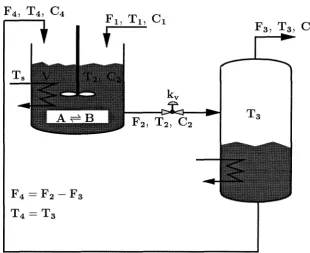
3.8 Example: Continuous Stirred Tank Reactor (CSTR)

+

Flash Unit 96

3.8.l Description of the system 96

3.8.2 CSTR

+

flash dynamics 98

3.8.3 Computation of steady states 99

3.8.4 Simulation results . . . 102

4

Output Feedback Contractive NLMPC: Nominal Case 106

4. 2.1 Basic stability definitions . 4.2.2 Basic assumptions

4.2.3 Stability analysis .

4.3 Dynamic observers for nonlinear systems 4.3.l Observer design . . .

4.3.2 Asymptotic convergence

4.4 MPC algorithm with state estimation . 4.5 Stability properties of contractive MPC +

nonlinear observer . . . . 4.6 Example: van der Vusse Reactor .

4.6.l van der Vusse reactor dynamics 4.6.2 Computation of steady states 4.6.3 Simulation results . . . .

109 110 111 118 118 122 129 131 134 134 137 138

5 Robust Output Feedback Contractive NLMPC: Parameter

Uncer-tainty

5.1 Introduction .

5.2 Stability of contractive MPC in the presence of bounded disturbances .

5.2.1 Basic assumptions

5.2.2 Stability analysis of Control Algorithm 1

5.3 Stability of MPC +state estimation scheme in the presence of param-eter uncertainty . . . .

5.3.1 Moving horizon formulation of the least squares estimation (LSE) procedure

5.3.2 Basic assumptions . . .

5.3.3 MPC with state estimation: implementation 5.3.4 Stability analysis of Control Algorithm 4 5.4 Mixed state/parameter LSE problem

5.4.1 Basic assumptions . . .

5.4.2 Properties of Estimation Procedure 3 190

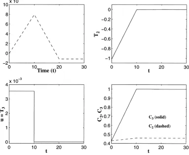
5.5 Example: Biochemical Reactor . . . . 197

5.5.1 Biochemical reactor dynamics 197

5.5.2 Computation of steady states 199

5.5.3 Simulation results . . . 201

6 Contractive NLMPC reformulated as a Quadratic Programming (QP) Problem

6.1 Introduction .

6.2 Contractive MPC posed as a QP 6.2.1 Description of the system

6.2.2 State feedback contractive MPC algorithm with linear approximation . . . .

6.2.3 Transforming the optimization into a QP 6.2.4 QP format . . . . 6.2.5 Basic philosophy of the controller design 6.3 Stability analysis of Control Algorithm 5 . . . .

6.3.1 Basic assumptions for the state feedback controller 6.3.2 Stability results for the state feedback MPC controller 6.3.3 Output feedback contractive MPC algorithm with

linear approximation 6.4 Examples . . . .

6.4.1 Example 1: A Nonholonomic System (Car) . 6.4.2 Comparison between contractive MPC with local

linearization and Astolfi's discontinuous controller (unconstrained case) . . . .

6.4.3 Example 2: Continuous Stirred Tank Reactor (CSTR)

+

Flash Unit . . . .

6.4.4 Example 3: 2-Degree of Freedom Robot

6.4.5 Example 4: Fluid Catalytic Cracking Unit (FCCU)

6.4.6

Bibliography

Example 5: van der Vusse Reactor 308

List of Figures

2.1 Inherent structure in all MPC schemes. 2.2 Optimization problem at time k. . .

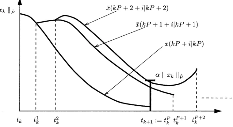
3.1 P control problems for a fixed k. Predicted trajectories generated by contractive MPC for a fixed k and j varying in the interval j = O, ... ,P-l . . . .

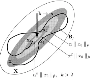
3.2 Exponential decay of the state trajectory ..

3.3 State trajectory generated by the contractive MPC scheme ..

3.4 Discrete and continuous-time exponentially decaying upper bounds for 19

20

51

51

52

the state trajectory. . . 54

3.5 Coordinate system for the car. 63

3.6 Resulting paths in the xy-plane using CNTMPC when the car is ini-tially on the unit circle and parallel to the x-axis. . . . 65 3. 7 Resulting paths in the xy-plane using the analytic discontinuous

con-troller when the car is initially on the unit circle and parallel to the x-axis.

3.8 Car: State and control responses for SNLMPC and CNTMPC in the 66

unconstrained case. . . 68 3.9 Car: State and control responses for SNLMPC and CNTMPC in the

constrained Case 1. . . 69 3.10 Car: State and control responses for SNLMPC and CNTMPC in

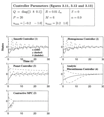
con-strained Case 2. . . 71 3.11 Car: Comparison of CNTMPC with other classic controllers for

non-holonomic systems (state response). . . 72 3.12 Car: Comparison of CNTMPC with other classic controllers for

3.13 Car: Comparison of CNTMPC with other classic controllers for

non-holonomic systems (plots in the xy-plane). 74

3.14 Schematic diagram of the FCCU. . . 75 3.15 FCCU: State and control responses for SNLMPC/CNTMPC in the

unconstrained Case 1 (Transition 1). . . 83

3.16 FCCU: State and control responses for SNLMPC in the unconstrained

Case 2 (Transition 1). . . 84

3.17 FCCU: State and control responses for SNLMPC in the unconstrained

Case 1 (Transition 2). . . 86

3.18 FCCU: State and control responses for SNLMPC in the unconstrained

Case 2 (Transition 2). . . 87

3.19 FCCU: State and control responses for CNTMPC in the unconstrained case (Transition 2). . . 88

3.20 Top view and cross section of the robot. 90

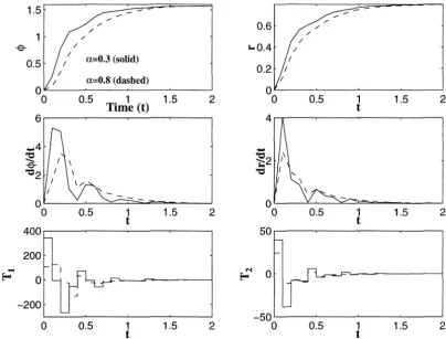
3.21 The robot workspace. . . 91 3.22 Robot: State and control responses for SNLMPC and CNTMPC in

the unconstrained Case 1. . . 92 3.23 Robot: State and control responses for SNLMPC and CNTMPC in

the unconstrained Case 2. . . 94 3.24 Robot: State and control responses for SNLMPC and CNTMPC in

the constrained case. . . 95

3.25 Schematic diagram of the CSTR and fl.ash unit. 96

3.26 CSTR

+

Flash: State and control responses Case 1. 103 3.27 CSTR

+

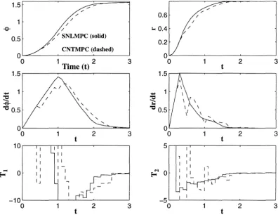
Flash: State and control responses in Case 2. 105

4.1 Schematic representation of the van der Vusse reactor. . . 135 4.2 van der Vusse CSTR: State and control responses for SNLMPC and

CNTMPC in the unconstrained Case 1. . . 139 4.3 van der Vusse CSTR: State and control responses for SNLMPC and

4.4 van der Vusse CSTR: State and control responses for SNLMPC and CNTMPC in the unconstrained Case 3. . . 142 4.5 van der Vusse CSTR: State and control responses for CNTMPC in the

constrained case. . . 144 4.6 van der Vusse CSTR: State and control responses for SNLMPC and

CNTMPC in the unconstrained case and under exponentially decaying disturbance d1 . . . 146 4. 7 van der Vusse CSTR: State and control responses for SNLMPC and

CNTMPC in the unconstrained case and under exponentially decaying disturbance d2 . . . . • . . . . • • . . . 147 4.8 van der Vusse CSTR: State and control responses for SNLMPC and

CNTMPC in the constrained case and under exponentially decaying disturbance d2 . . . . • . • . . . • . . . 148 4.9 van der Vusse CSTR: State and control responses for SNLMPC and

CNTMPC in the unconstrained output feedback case. . . 151 4.10 van der Vusse CSTR: State and control responses for SNLMPC and

CNTMPC in the constrained output feedback case. . . 152

5.1 Schematic representation of a continuous bioreactor with substrate in-hibition. . . 197 5.2 Bioreactor: State and control responses in Case 1.1 (Transition 1). 204 5.3 Bioreactor: State and control responses in Case 1.2 (Transition 1). 205 5.4 Bioreactor: State and control responses in Case 1.3 (Transition 1). 207 5.5 Bioreactor: State and control responses in Case 1.4 (Transition 1). 209 5.6 Bioreactor: State and control responses in the constrained Case 2.1

(Transition 1). . . 210 5.7 Bioreactor: State and control responses in the constrained Case 2.2

5.10 Bioreactor: State and control responses in Case 1.3 (Transition 2). 217 5.11 Bioreactor: State and control responses in Case 1.4 (Transition 2). 218 5.12 Bioreactor: State and control responses in the unconstrained output

feedback nominal case using EKF (Transition 2). . . 220 5.13 Bioreactor: State and control responses in the unconstrained output

feedback robust case using EKF (Transition 2). . . . 221 5.14 Bioreactor: State and control responses in the output feedback robust

case using LSE (Transition 2). . . . 223

6.1 P control problems for a fixed k. Predicted trajectories generated by the robust contractive MPC scheme for a fixed k and j varying in the interval j = 0, ... , P - 1. . . 255 6.2 Next P control problems at k

+

1. Predicted trajectories generated

by the robust contractive MPC scheme at k

+

1 and j varying in the interval j = 0, ... , P - L . . . ..

6.3 State trajectories generated by the contractive MPC scheme.

6.4 Resulting paths in the xy-plane using contractive MPC with local linearization when the car is initially on the unit circle and parallel to

256 257

the x-axis. . . 283 6.5 Resulting paths in the xy-plane using contractive MPC with local

linearization when the car is initially on the unit circle and parallel to the x-axis. . . 284 6.6 Resulting paths in the xy-plane using the analytical discontinuous

controller when the car is initially on the unit circle and parallel to the

x-axis. 286

6. 7 Car: State and control responses and xy-plot generated by standard MPC with local linearization in the constrained case. . . 288 6.8 Car: State and control responses and xy-plot generated by contractive

6.10 CSTR

+

Flash: State and control responses in the constrained Case 2. 293 6.11 CSTR

+

Flash: State and control responses in the constrained Case 3. 295 6.12 Exponentially decaying disturbances used in the simulations shown in

figure 6.11. . . 296 6.13 Robot: State and control responses in Case 1. . 297 6.14 Robot: State and control responses in the constrained Case 2. 299 6.15 FCCU: State and control responses in the unconstrained Case 1.1. 300 6.16 FCCU: State and control responses in the unconstrained Case 1.2. 302 6.17 Exponentially decaying disturbances used in the simulations shown in

figure 6.16. . . 303 6.18 FCCU: State and control responses in the unconstrained Case 1.3. 304 6.19 FCCU: State and control responses in the unconstrained Case 2.1. 305 6.20 FCCU: State and control responses in the unconstrained Case 2.2. 307 6.21 van der Vusse CSTR: State and control responses in the constrained

Case 1.1. . . 309 6.22 van der Vusse CSTR: State and control responses in the unconstrained

Case 1.2. . . 310 6.23 van der Vusse CSTR: State and control responses in the constrained

Case 1.3. . . 311 6.24 van der Vusse CSTR: State and control responses in the constrained

Case 1.4. . . 313 6.25 van der Vusse CSTR: State and control responses in the constrained

Chapter 1 Introduction

The vast majority of industrial processes is typically operated using linear controllers, although it is well known that many of these processes are highly nonlinear. The major difficulty in the design of feedback control laws for nonlinear systems arises from the necessity to explore the whole state space. The problem of the design of feedback controls for nonlinear systems has found a general solution only in the case of systems which are feedback equivalent to linear systems. The fact that most nonlinear systems are not feedback equivalent to linear ones has motivated the study of alternative control techniques which do not require construction of diffeomorphic state-feedback transformations. One of these techniques is model predictive control (MPC) - an optimal control based method for the construction of stabilizing feedback control laws.

A key feature contributing to the success of model predictive control is that var-ious process constraints can be incorporated directly into the on-line optimization performed at each time step. In other words, model predictive control has the poten-tial, not easily possessed by other methods, to globally stabilize linear and nonlinear systems subject to control and/ or state constraints. This is undoubtedly a very im-portant feature since many practical control problems are dominated by constraints. In [89], Mayne and Polak state:

"It can be argued that the most urgent, unresolved control problem is an effective, practical method for the design of feedback controllers for

constrained dynamic systems, linear or nonlinear."

(MIMO) systems with very little changes in the formulation compared to the single-input single-output (SISO) case, and its variable structure in the event of faults.

Besides being subject to input/state constraints, most real systems are represented by process models which are not accurate. Furthermore, they are invariably subject to disturbances of various kinds. Due to these practical problems, it is important for the controllers designed to be robust (i.e., take into account the model/plant mismatch which may exist and guarantee satisfactory stability and performance properties of the closed-loop system) and present good disturbance rejection properties.

Regarding robustness, a very extensive theory [102] has been developed for the robust control of linear systems without constraints. This theory has been proven successful when applied to a number of academic case studies such as, e.g., high purity distilla-tion columns (see [116)), with process constraints not taken into consideradistilla-tion. The neglect of constraints has made this robust control theory unsuitable for industrial applications. When constraints are considered, even if the plant is linear, the overall control problem becomes nonlinear and this is the reason why constrained problems are so much harder to deal with than unconstrained ones.

In spite of MPC's considerable practical importance and extensive use, there is in fact very little theory to guide the design and tuning of these controllers for stability, performance and robustness, especially in the nonlinear case. Moreover, the exist-ing stability and robustness analysis of MPC applied to nonlinear systems is rather complicated and non-intuitive and the resulting controllers hardly implementable.

1.1

Motivation

Most practical control problems are dominated by process constraints and nonlin-earities. The most common process constraints are constraints on the manipulated and/ or state variables. Regarding the nonlinear character of most real systems, non-linearities can be quantified as "weak" or "strong" (see [5, 6]) and it may be that while a linear controller design is satisfactory for a "weakly nonlinear" system it will most probably be inappropriate for a system with stronger nonlinearities.

With respect to process constraints, constraints on the manipulated variables are present in the vast majority of processes and they result from physical limitations of the actuators which cannot be exceeded under any circumstances. Safe operation of a plant very often requires limitations on states as well, such as velocity, accelera-tion, temperature and pressure. State constraints are also a natural way to express control performance objectives in many applications. Although most control con-straints should be respected throughout the operation (hard concon-straints), it may be unavoidable to exceed the state constraints for some time, especially if the system is subjected to disturbances not accounted for in advance. Therefore, the constraints imposed on states and output variables are most often soft constraints.

A rich theory has been developed to address the robustness issue in unconstrained linear systems (as will be discussed in the next section). For constrained and uncertain linear systems the scope of results is not so vast. And, as one would expect, for constrained and uncertain nonlinear systems results are few and incomplete. One can surely say that the theory on constrained control of nonlinear systems (be it the nominal or robust case) is still in its infancy. It is the goal of this thesis to add a contribution to this area.

1.2

Previous work

1.2.1

A general look

Open-loop optimal feedback, dating back to a 1963 seminal paper by Propoi, [108], is a general approach for the construction of stabilizing feedback laws for systems subject to input constraints and other nonlinearities. Originally, it was based on the idea that in a sampled-data system, the control to be applied between sampling times can be determined by solving a fixed horizon open-loop optimal control problem with or without constraints. Over the years, open-loop optimal feedback has been explored under the names of model predictive control (to mention a few references, see [48, 49, 50, 51, 73, 94, 107]) and moving horizon control (see, e.g., [62, 68, 69, 71, 81) 82, 83, 84, 85, 95]).

The literature dealing with linear MPC presents an enormous amount of results on issues such as stability, reference trajectory tracking and constant disturbance rejec-tion capabilities of the resulting feedback systems, under the assumprejec-tion that control and state variables are unconstrained (see, e.g., [33]). Nominal stability results for constrained linear systems can be found in [31, 101, 91, 109], for robust analysis see [66, 122, 127].

a naive application of the strategy can lead to instability. The early literature dealt with the stabilizing properties of moving horizon control laws based on open-loop optimal control for finite horizon optimal control problems with quadratic criteria and no input constraints. More recently, [66, 69, 71, 128] dealt with linear time-varying (LTV) systems, [1, 2, 3, 62, 92, 91] dealt with nonlinear discrete-time systems and [28, 81, 82, 83, 84, 85] have established the stability properties of nonlinear, continuous-time systems with moving horizon control in the presence of constraints. In [95] Mayne and Michalska examined the robust stability of a moving horizon control, although the analysis is somewhat involved and the resulting hybrid control law (a nonlinear MPC controller is used to drive the states to a small neighborhood of the origin and the control law switches over from MPC to a linear controller which is then used to drive the states asymptotically to the origin) is hard to implement even for simple examples. [83, 85] took into account the non-trivial time needed for the computation of the open-loop control law even in the nominal case. [125] analyzed the robust stability problem by discretizing the problem into multiple linear feedback control systems.

Dealing with the nonlinear control and estimation problems simultaneously we can find [87], although the stability analysis presented in that work is quite complicated and incomplete.

1.2.2

MPC and its different implementations

The basic formulation of an MPC problem for a nonlinear plant of the form

is the following:

subject to:

j;P(t)

y(t)

fP(xP(t), u(t), t), xP(to)

=:

Xb

gP(xP(t), u(t), t)

min <I>[x(t),

u(t)]

u(t)

(1.1) (1.2)

(1.3)

x(t)

=

f

(x(t), u(t), t),

with

_x(t0)

=

x0

and

t

E

[t

0 ,

t0

+PT]

(1.4)

where:

K,(x(t), u(t), t)

= 0 (1.5)

h(x(t), u(t), t) ;:::

0 (1.6)

<I> := performance criterion (a positive definite function)

J,

JP

:= model and plant dynamics, respectively

gP

:= output model

K,,

h := equality and inequality time-varying mixed input/state nonlinear constraints (in the most general case), respectively

xP(t)

:= state vector of the plant

y(t)

:= output vector

u(t)

:= control vector

P := prediction horizon; an integer number which can be finite or infinite

xg, x

0 := initial condition of the plant and model states, respectively

t₀ := initial time of computation

T := sampling time

PT := prediction time

Throughout this thesis the symbol ":=" means that the left-hand side is defined to be equal to the right-hand side; the reverse holds for "=:".

The control sequence

u(t)

is computed for

t

E

[t

0 ,

t

0 +PT] but only

u(t)

restricted to t E [t0 , ti := t0

+

T] is actually applied to the real plant (1.1). At time ti a

measurement y(ti) is obtained, the states of the plant are estimated (in the case where not all states can be directly measured at sampling times) and with this new initial condition Xi := x(ti) (where x(t) represents the estimated States of the plant at time

t)

a new optimization problem is solved at time ti. This is known as a receding horizon implementation of the control law.

The plant (1.1) is linear if its dynamics is given by:

j;P (

t)

y(t)

jP(xP(t), u(t),

t) :=

AP(t)xP(t)

+

BP(t)u(t)

CP(t)xP(t)

+

DP(t)u(t)

(1.7) (1.8)

If all the matrices

AP(t), BP(t), CP(t)

and

DP(t)

are constant, the linear system (1.7), (1.8) is said to be time-invariant (LTI system); if one or more of them vary in time, we have a linear time-variant (LTV) system.

x(t)

=

j (x(t), u(t),

t) :=

A(t)x(t)

+

B(t)u(t)

(1.9)

If

j(x(t), u(t), t) ( {A(t), B(t)})

differ from

fP(xP(t), u(t), t) ( {AP(t), BP(t)})

for some

t

E

[t

0 , oo) we have a nonlinear (linear)

robust

control problem at hands.

In general, the performance criterion <I> is given by:

<J>[x(t), u(t)]

:= {tp:=to+PT

<,b[t, x(t), u(t)]dt

+

cp[to, x(to), tp, x(tp )]

(1.10)

lt0

where the functions ¢ :

R

x

Rn

x

Rm --+ R

and cp :

R

x

Rn

x

R

x

Rn --+ R

are positive (semi-)definite functions of their arguments.

Most commonly, ¢is a time-invariant quadratic function of its arguments, i.e.,

<,b[t, x(t), u(t)]

=

x(t)' Qx(t)

+

u(t)' Ru(t)

with Q, R positive definite matrices, and cp = 0.

Within the context of the preceding formulation, MPC algorithms can be divided into the following main categories:

(1) Finite prediction horizon [PE (0, oo)] for:

• Linear plants [27, 35, 49];

• Nonlinear plants [19, 20, 39, 48];

(2) Infinite prediction horizon

[P--+

oo] for:

(3) Finite prediction horizon with end constraints1 (also known as stability con-straints) for:

• Linear plants [13, 23, 32, 52, 69, 101, 122, 123, 127];

• Nonlinear plants [1, 2, 28, 62, 63, 81, 82, 83, 84, 85, 91, 95, 96, 124].

In the first category a simple finite horizon objective function is employed which does not, per se, guarantee stability. This means that closed-loop stability cannot be assumed simply because the on-line optimization finds a solution. The issue of closed-loop stability is complicated by two facts: first, there is always uncertainty associated with the model used in the prediction; second, the presence of constraints in the optimization problem results in a nonlinear closed-loop system even if the model and plant dynamics are linear. In [22] the authors underlined the poor stability properties of finite prediction horizon schemes.

In the second category, [92, 109] propose a control algorithm which minimizes an infinite horizon objective function subject to the constraint that the unstable modes of the plant are set to zero at some finite time. This kind of control algorithm has desirable stability properties in the nominal case but it cannot be extended in a straightforward manner to plants with uncertainty. In [66], the authors propose a technique which deals explicitly with model/plant uncertainty in LTV plants. The goal in this technique is to design, at each time step, a state feedback control law which minimizes a "worst-case" infinite horizon objective function, subject to con-straints on the control inputs and plant outputs. The problem of minimizing an upper bound on the "worst-case" objective function subject to constraints is reduced to a convex optimization involving linear matrix inequalities (LMis). It is shown that the feasible receding horizon state feedback control design robustly stabilizes the set of uncertain plants. In [1, 3], discrete-time nonlinear systems are considered and global stability of the infinite prediction horizon scheme is shown under certain stabilizability assumptions.

It should be pointed out that one of the great restrictions of infinite prediction horizon schemes (even with finite control horizons) is naturally computational.

The third category is the one with most of the desirable stability and robustness characteristics. In the nonlinear context, MPC for discrete-time systems with mixed state/control constraints is discussed in an important paper by Keerthi and Gilbert [62]. The control action is determined by minimizing, at each kth time step, a

non-linear cost function over the horizon [k, k +Pk] (here the horizon P is not constant, instead it is included as a decision variable in the optimization together with the con-trol and represented by Pk) subject to the mixed state/control constraints and the terminal equality constraint x( k

+

Pk

I

k)

=

0 and setting the current control equal to the first element of the minimizing sequence. Keerthi and Gilbert show that this con-trol is, under certain conditions, stabilizing. The finite horizon approach for nonlinear discrete-time systems proposed in [1, 2] is very similar to this found in [62], the only apparent difference being that certain observability assumptions on the system can be relaxed because the performance criterion is defined in terms of states and inputs (instead of outputs and inputs as in [62]). In [91] the same end equality constraint is used to show stability using Lyapunov arguments. The authors show in that paper that systems which are feedback linearizable can be asymptotically stabilized with MPC. They also find discrete-time systems which cannot be stabilized with contin-uous feedback and they show that MPC generates a discontincontin-uous feedback which stabilizes such systems.

value function is required, allowing for less strict assumptions on the behavior of the linearized system. In each case, the finite horizon control requires exact solution, at each time instant k, of a finite horizon nonlinear control problem with the terminal equality constraint x(k

+

Pklk) = 0.

In [82] a relaxed version of the stability constraint for continuous-time nonlinear systems is presented, i.e., instead of x(k+Pklk)

=

0, the authors use x(k+Pklk) E W

(where W is some neighborhood of the origin). Since the terminal constraint has been relaxed, the MPC strategy loses its stabilizing properties inside W. To compensate for this effect, a linear, locally stabilizing controller designed for the linearized system is used inside W. The resulting "hybrid" controller is shown to be globally stabilizing.

One common factor in the stability proofs of all MPC schemes mentioned here is that the questions related to feasibility are eluded through the assumption that the constrained control problem always remains solvable. In [113], it is argued that the issue of feasibility is in fact central to the question of stability and that, therefore, the feasibility assumption is inappropriate. In that work, a technique for systematic handling of infeasibilities is proposed which is such that its use allows stability guar-antees obtained under the assumptions of feasibility to be carried over to the usual case when feasibility cannot be guaranteed (details of this technique are not found in [113] but the authors claim that they will be published in the Ph.D. thesis of P. Scokaert).

1.3

Thesis overview

1.3.1

General contents

In chapter 2, we give a brief tutorial review of the state space formulation of MPC for both linear and nonlinear systems. There we concentrate on the stability results found in the literature for the three main classes of linear/nonlinear constrained MPC controllers:

(1) Finite prediction horizon MPC.

(2)

Infinite prediction horizon MPC.

(3) Finite prediction horizon MPC with (stabilizing) end constraints.

We see that for class (1) there are no stability guarantees. For class (2) the controller is stabilizing if the optimization is feasible. And, finally, for class (3), even though the prediction horizon is finite, the end constraints add stability (and sometimes robustness) to the controller.

In chapter 3, we introduce our so-called Contractive MPG scheme. Contractive MPC is a finite horizon nonlinear MPC algorithm which is stabilized through the addition of an end constraint called contractive constraint. In that chapter, we introduce the formulation, implementation and basic philosophy of the contractive MPC scheme and discuss its stability properties in the nominal case and in the absence of disturbances. The results show that the contractive constraint exponentially stabilizes the closed-loop system when model uncertainty and disturbances are absent. We also discuss the conditions under which the chosen standard quadratic objective function is a Lyapunov function for the closed-loop system. Finally, four examples are introduced:

(2)

A fluidized catalytic cracking unit (FCCU)

(3) A 2-degree of freedom robot

( 4) A continuous stirred tank reactor (CSTR)

+

flash unit

We apply our contractive MPC scheme to these four examples which are of very dif-ferent natures and present varied levels and sources of difficulties (that are discussed there) and the obtained simulation results are compared with a standard finite pre-diction horizon nonlinear MPC algorithm. Moreover, in the case of the car, we also present a comparison of our results with some analytical control design techniques derived especially for nonholonomic systems.

In chapter 4, we examine how the stability results are modified when the system is subjected to an asymptotically decaying disturbance of bounded energy. Our results demonstrate that the closed-loop system becomes uniformly asymptotically stable in the presence of this class of disturbances (thus, the exponential stability properties of contractive MPC are weakened to uniform asymptotic stability). We also show that this kind of disturbance can be caused by introduction of an asymptotically conver-gent observer into the closed-loop for purposes of state estimation. We then derive sufficient conditions under which the association of an exponentially stable controller (such as contractive MPC) with an asymptotically convergent observer, generates an asymptotically stable closed-loop system. Furthermore, we design such an observer for a continuous-time system with discrete observations and prove its asymptotic con-vergence properties. The results reveal that if the outputs are measured continuously, then this nonlinear observer has its convergence properties strengthened as it becomes exponentially stabilizing.

nonlin-ear state estimator proposed in that chapter (the reason we use this discrete version of the observer instead of the original mixed continuous/discrete one is to reduce the differential Riccati equation to an algebraic Riccati equation) for the example men-tioned above and examine the behavior of the closed-loop system generated by the resulting output feedback controller.

In chapter 5, we first look into the state feedback control problem when persistent, bounded and non-additive disturbances affect the nonlinear dynamics of the system. In the nonlinear context, the problem posed by disturbances of this kind is equiva-lent to having parameter uncertainty only (i.e., model and plant are matched in the nonlinear structure, only some - or all - parameters are unknown). We demonstrate that the most which can be guaranteed under non-additive bounded disturbances or constant parameter mismatch, is that the states are driven to a control invariant set whose size is proportional to the magnitude of the disturbances or parameter devia-tion. Then, we examine how these results change when the states are also unknown (which constitutes the output feedback case) if the parameters are unknown but con-stant. We use a moving horizon-based least-squares estimator for state estimation. Additionally, we study in that chapter how the results are modified if both states and parameters are unknown, the parameters are time-varying, the system is subjected to additive disturbances and the moving horizon least-squares estimation procedure seeks to estimate states, disturbances and parameters.

The example used to test the robust state and output feedback contractive MPC controllers proposed in chapter 5 is a biochemical reactor with substrate inhibition. There we study how the closed-loop behaves when there is a constant parameter deviation between the model used for prediction, computation of the contractive constraint and estimation and the real nonlinear system.

optimization problems. Indeed there is no general agreement on the best approach to be used for its solution and much research is still to be done. Due to the difficulties inherent to solving nonlinear programming problems and since MPC requires the opti-mal (feasible) solution to be computed on-line, we propose in chapter 6 an alternative implementation which guarantees that the problem can be solved in a finite number of steps. It is well-known that quadratic programming (QP) problems satisfy this requirement. Thus, we show in that chapter how to pose the optimization problem as a QP by means of using a linear approximation of the original nonlinear system in the prediction step of the MPC control algorithm and by implementing the contractive constraint in an appropriate way. We propose three different ways of implementation of the contractive constraint, namely, the "approximate (or conservative) approach", the "penalty function approach" and the "approach based on sensitivity analysis of the QP". We also show how to pose the problem as a QP by appropriately defining the Hessian matrix, the gradient vector and the constraint matrices.

Still in chapter 6, we describe the formulation, implementation and basic philosophy of this computationally simplified but harder to analyze controller. The reason why the analysis of the contractive MPC controller, under the local linear approximation of the original nonlinear system, becomes more involved, comes from the fact that the linearization introduces a structural mismatch between the plant and the model used in the control computations (it is basically a linear/nonlinear mismatch, if no other types of uncertainties are considered). Therefore, the controller must be robust with respect to this mismatch (i.e., the controller must stabilize the states of the plant even though nonlinearities are ignored in the prediction). Under certain assumptions on this model/plant mismatch (a growth condition on the nonlinear terms of the model), we show that the states of the plant can be driven to a control invariant set whose size depends on how "strongly nonlinear" the system is. We also include bounded disturbances and parameter mismatch in this analysis.

the nonholonomic system/ car, the FCCU, the CSTR

+

flash unit (all of these intro-duced in chapter 3) and the van der Vusse reactor(introintro-duced in chapter 4) and we compare the results with the ones previously obtained for when the nonlinear system itself is used in the prediction step of the MPC control algorithm.

1.3.2 List of theorems in the thesis

Chapter 3 State Feedback Contractive NLMPC: Nominal Case

Theorem 3.1 Exponential stability of the closed-loop system.

Theorem 3.2 Conditions for the objective function to be a Lyapunov function

for the closed-loop (not necessary for exponential stability).

Chapter 4 Output Feedback Contractive NLMPC: Nominal Case

Theorem 4.1 Uniform asymptotic stability of the closed-loop system in the

presence of asymptotically decaying disturbances in the state feedback case.

Theorem 4.2 Feasibility condition (sufficient condition on the magnitude of

the asymptotically decaying disturbances so that feasibility can be as-sured).

We then discuss how these asymptotically decaying additive disturbances can be caused, for example, by introduction of an asymptotically stable state estimator into the closed-loop. We propose a mixed continuous/discrete-time nonlinear observer and examine its stability properties.

Theorem 4.3 Computation of a stability region for the nonlinear observer

Theorem 4.4 Closed-loop stability in the output feedback case. The

associa-tion of the asymptotically convergent nonlinear observer proposed in this chapter with the exponentially stabilizing contractive MPC controller is shown to originate an asymptotically stable closed-loop.

Chapter 5 Robust Output Feedback Contractive NLMPC: Parameter Uncertainty

Theorem 5.1 Computation of a bound on the difference between model and

plant states at the end of prediction horizons, in the presence of parameter uncertainty and in the state feedback case.

Theorem 5.2 Stabilizing properties of the state feedback controller in the

pres-ence of parameter uncertainty.

Theorem 5.3 Feasibility condition (sufficient condition on the magnitude of

the parameter uncertainty so that feasibility can be assured).

Theorem 5.6 Computation of a bound on the difference between true and

esti-mated states in the presence of parameter uncertainty. The state estimator is a moving horizon-based least squares estimation (LSE) procedure.

Theorem 5. 7 Stabilizing properties of contractive MPC in the presence of

parameter uncertainty and in the output feedback case.

Theorem 5.8 Feasibility condition (sufficient condition on the magnitude of

the parameter uncertainty so that feasibility can be assured in the presence of state estimation errors).

Theorem 5.9 Using the LSE moving horizon-based procedure for both state

Chapter 6 Contractive NLMPC reformulated as a Quadratic Programming (QP)

Problem

Here, local linear approximations of the nonlinear system are used for predic-tion and in the computapredic-tion of the contractive constraint, in order to reduce the optimization to a simple QP problem. Thus, we proceed to show how the stabil-ity properties of the closed-loop are modified when this structural model/plant (linear/nonlinear) mismatch is introduced. The presence of disturbances and parameter uncertainty is also taken into consideration in our results.

Theorem 6.2 Computation of a bound on the difference between the states

of the nonlinear system and of its local linearization at the beginning of prediction horizons.

Theorem 6.3 Feasibility condition (sufficient condition on the structural

model/plant mismatch and on the magnitude of possible parameter un-certainty and disturbances, so that feasibility can be assured).

Theorem 6.4 Derivation of finite bounds on the norm of the continuous state

trajectory generated by the controller for all time t

2:

0, demonstrating its well-posedness.

Theorem 6.5 Feasibility conditions for systems with stable Jacobian in the

whole state space (derivation of a lower bound on the contractive parameter so that feasibility can be assured) in the absence of parameter uncertainty or disturbances.

Theorem 6.6 Stability and feasibility properties of the output feedback scheme

Chapter 2

MPC: An Overview

2.1

Implementation aspects

A tutorial review of the state space formulation of Model Predictive Control for both linear and nonlinear systems is presented in this chapter.

The various implementations of MPC are identical in their global structure but differ in the details. The general structure of MPC schemes is shown in figure 2.1.

Reference

u y

Optimizer _Plant

,__ _ __._. 0 bserver

Figure 2.1: Inherent structure in all MPC schemes.

The selected observer uses the input and output information ( u and y, respectively) and computes the state estimate

x.

With this estimate, one can use an optimization scheme to predict the trajectory of the controlled variables y over some prediction (or output) horizon P with the manipulated variables u changed over some control (or input) horizon M (M

:SP).

This prediction step is represented in figure 2.2.

•

•

Past Future

•

•

k k+l

Reference Trajectory r

- - - . - --+- ---·--·-

----•

•

Predicted Outputs y(k +ilk)

Manipulated Inputs u(k +ilk)

k+M-1 k+P

~--Control Horizon ""

[image:36.515.83.426.59.331.2]

- - - Prediction Horizon >

Figure 2.2: Optimization problem at time k.

the selected reference trajectory in a satisfactory manner. The optimizer takes into account the input and output constraints which may exist, by incorporating them directly into the optimization. For linear systems, if a linear or quadratic objective function is considered, the resulting optimization is a linear or a quadratic program-ming problem, respectively. For nonlinear systems, independent of the chosen perfor-mance criterion, the optimization becomes a nonlinear programming problem which is non-convex in the majority of cases.

values of the horizons M and P are generally finite. However, it has been observed that it is very hard to provide stability guarantees for an MPC scheme with finite output horizon P (see [22]). Stability results can be obtained when P is infinite, keeping M finite. It has been shown that such selection of controller parameters makes it possible to guarantee certain stability properties of the closed-loop system while keeping the computation effort reasonable in most cases.

2.

2

Basic formulation

A very general and not very detailed formulation of the prediction step in MPC algorithms was given in chapter 1. Here we will go into more details regarding the shape of the objective function, prediction models, state estimators and constraints.

2.2.1

Prediction models

(1)

Continuous-Time Systems

Linear: In its most general form, a linear prediction model is given by:

±(t)

y(t)

A(t)x(t)

+

B(t)u(t)

+

E(t); x(O)

=:

x

0 given

C(t)x(t)

+

D(t)u(t)

(2.1) (2.2)

where

x(t)

E

Rn

denotes the state at time

t, u(t)

E

Rm

the manipulated variables (or inputs) and

y(t)

E RP the controlled variables (or outputs). Here we have not included the disturbance or the noise that the actual plant may be subjected to,

time-varying (LTV), if they are all constant we have a linear time-invariant (LTI) system.

Nonlinear:

±(t)

y(t)

f

(x(t), u(t), t); x(O) = x0 given

g(x(t), u(t), t)

(2.3)

(2.4)

In most cases, the nonlinear system is time-invariant, that is,

f (.) :

Rn x Rm x R -+ Rn and g(.) : Rn x Rm x R -+ RP are not explicit functions of time. Usually,

f

and g are assumed to be continuously differentiable functions.

(2)

Discrete-Time Systems

Linear:

x(k

+

1)

y(k)

<I>(k )x(k)

+

f ( k )u( k)

+

rJ( k); x(O), u(O) given (2.5)

C(k)x(k)

+

D(k)u(k) (2.6)

The matrix <I> ( k) is known as state transition matrix.

When the continuous-time linear system (2.1) is time-invariant, the dis-crete form (2.5) can be easily obtained from that system by having <I>(k),

r(k), rJ(k) given by:

<I>(k)

·-f(k)

·-rJ(k)

·-where T is the sampling time.

eAT

T

lo

eA(T-t) Bdt

for eA(T-t) Edt

(2.7)

(2.8)

Nonlinear:

x(k

+

1)

y(k)

F(x(k), u(k), k); x(O), u(O) given

G(x(k), u(k),

k)

(2.10)

(2.11)

In general, it is not possible to obtain a closed form solution of a general continuous-time nonlinear system as given by (2.3) (the solution has to be computed numerically), which means that F and G are not know explicitly for most systems modeled originally in continuous-time form.

2.2.2

State estimators

In general, state estimators have the following form:

Continuous-Time Systems:

±(t)

y(t)

Discrete-Time Systems:

i(k)

y(k)

f

(x(t), u(t),

t)

+

K(t) [y(t) - y(t)]

g(x(t), u(t), t)

F(x(k), u(k), k)

+

K(k)

[y(k) -

y(k)]

G(x(k), u(k), k)

(2.12) (2.13)

(2.14) (2.15)

In the case where

J (.)

is continuous (discrete) and linear, either because the plant is linear or because we are using a linearized estimator for a nonlinear plant, K ( t) (or

2.2.3

Objective function

Various objective functions can be chosen depending on one's goal in using MPC. The most common one applies the 2-norm both spatially and temporally.

For continuous-time systems the following objective function is commonly used:

(2.16)

where

II . II

denotes the Euclidean norm of a vector and

II

x

lip:=

V

x' f>x, with

f> E

Rnxn

positive definite, is the weighted Euclidean norm of x E

Rn.

II .

/I

also

denotes the Euclidean norm of a matrix. More generally,

II .

llP,

p

2:

1, denotes the Holder or p-norm of a vector or matrix (note that when p = 2 the p-norm becomes the Euclidean norm) and is given by:

II

x

llp

1

·- (lx1IP

+ ... +

lxnlP)iJ,

\::/x E

Rn,

p

2:

1

II

A

lip ·-

sup II Ax /IP \::/A E

Rmxn

x:fO, xE~n

/I

X I Ip '

where

lxil

denotes the absolute value of xi E R, Vi= 1, ... , n.

(2.17) (2.18)

If we make p = 2 in definition (2.18) and

A

E

Rnxn ( cnxn,

in the general case of complex matrices and vectors) we have the so-called induced (matrix) norm of A corresponding to the Euclidean vector norm II .

II

on

Rn

(Cn):

II

A

II:=

sup

x,tO, xE~n

II

Ax

II

II

x

II

llxll=l sup

ii

Ax II = ilxll:Sl sup 11 Ax 11 (2.19)

[54, 58]).

Besides the Euclidean and Holder norms of vector and matrices, we will define

Ill . Ill

to be the induced norm on tensors. Let

II . II

be a given norm on Rn (en). Then, for each tensor

t

E Rnxnxn (TE cnxnxn), the quantity 111t111 defined by

lllTlll ·-

sup x,y#O, x,yEfRn

II y'i'x II

II

Y

1111

x

II

llxll=llYll=l sup

II

y'i'x

II

=

sup

llxll::;I, llYll9

II

y'i'x

II

(2.20)

is called the induced (tensor) norm of

T

corresponding to the vector norm II .

11-The notation used in (2.16) is the following: Xk are the states of the system at time

tk (in the output feedback case we would have ik, that is, the estimate of xk); to keep coherent with the discrete case, Pk is the output or prediction horizon (which is a decision variable, together with the control, in some algorithms and therefore we are allowing it to be a function of k); T is the sampling time; xk(t) represents the state trajectory of the model for all t E [tk, tk

+

PkT] given the initial condition

Xk at tk; uk(t) is the control trajectory to be computed for the same time interval and initial condition; Q and R are positive definite matrices and they are controller tuning parameters (known as weights in the objective function).

For simplified computation, most implementations of MPC generate a sequence of M 1 discontinuous control moves, { u(klk), ... , u(k

+

M -

llk)},

instead of a continuous trajectory uk(t). In other words, these controllers require that uk(t)

=

u(k+ilk) for all

t E [tk +iT, tk

+ (i+

l)T) and i E [O, M -1], and uk(t) = 0 fort E [tk +MT, tk +PkT].

In this case, the objective function can be rewritten as:

1 _{In the implementations where the output horizon is a decision variable there is no difference}

(2.21)

If the system is linear or has a closed form solution it is possible to express the states

xk(t)

and, consequently, the objective function, as an explicit function of the control moves.

From this point forward we will consider Pas a pre-specified tuning parameter, con-stant throughout the computations, in order to simplify the notation (unless otherwise necessary to make the distinction).

For discrete-time systems the most commonly used objective function is the quadratic one given by:

P M-1

Vi ·-

L

x(k + ilk)

1

Qx(k +ilk)+

L

u(k + ilk)1 Ru(k +ilk)+

i=l i=O

M-1

+

L

!:iu(k + iJk)' S!:iu(k +ilk) (2.22)

i=O

where:

S is a positive definite matrix

!:iu(klk) := u(klk) - u(k -

lJk - 1)

!:iu(k +ilk) := u(k + iJk) - u(k + i -

lJk),

i E

[1,

M -

1]

In general, one can choose the weights

Q, Rand

S to be time-varying (i.e. functions of k). For simplicity they are assumed to be time-invariant here.

advantages of using each of these, as well as some other special objective functions can be found in [26].

2.2.4

Constraints

The optimization or prediction step in MPC can be subject to general mixed state/control constraints of the form:

Equality Constraints:

ti:(x(t), u(t), t)

=

0 (2.23)

Inequality Constraints:

h(x(t), u(t), t) :::: 0 (2.24)

Inequality constraints are found much more often than equality constraints. In a nonlinear setting equality constraints can never be satisfied in a finite number of algorithm iterations and are therefore avoided.

In most MPC problem formulations, the only two types of constraints considered are input and state (in particular, output) constraints. The constraints on the input variables are in general hard constraints which impose lower and upper bounds on these variables, that is,

u(t) Eu:= {u E

Rm:

Umin::::; u::::; Umax}, Vt E

[O, oo)

(2.25)

To make the control problem meaningful U must contain the origin.

J.6.uj(k+ilk)J

s;

.6.umax,j,

Vi=

0, ... , M -l, k

2::

0, with .6.umax,j

>

0, Vj

=

1, ... , m (2.26)

where .6.uj(k

+

ilk),

.6.umax,j, j

=

1, ... , m, are the components of the vectors .6.u(k

+

ilk),

.6.umax, respectively. We will express these constraints in the follow-ing vector form:

J .6.

U ( k

+

i

I

k)

J

s;

.6.

Umax,

Vi =

0, ... , M - 1, k

2::

0,

.6.

Umax

>

0 (2.27)

where we have committed some abuse of notation since .6.u(k

+ilk)

is a vector and we have defined

I· I

to be a scalar norm. The reason for this notation is that we do not want the norm used here (which is linear in the components of the vectors .6.u(k

+

ijk))

to be confused with the 2-norm.

The output constraints are in general of the form:

Ymin

s;

y(k

+

i/k)

s;

Ymax, 'Vi= 1, ... , P, k

>

0 (2.28)

or in the "soft" format:

Ymin - E

s;

y( k

+ i

I

k)

s;

Ymax

+

E,

Vi

=

1, ... , P, k

2::

0 (2.29)

where <:: is an additional decision variable whose weighted quadratic norm is added to the objective function. This formulation allows the bounds Ymin and Ymax to be violated by at most E whenever the problem with hard constraints is not feasible. The

norm of E is added to the objective function so as to minimize the violation of these

In addition to input and output constraints, the optimization may be subject to physical constraints on the state variables (e.g., mole fractions have to lie between 0 and 1, temperatures in Kelvin degrees have to be always positive, concentrations are always non-negative, etc). Other useful state constraints are constraints imposed at the end of the (finite) prediction horizon known as end constraints. Some of these constraints are used, for example, to guarantee stability of the closed-loop as we will see later.

Two well-known "stabilizing" end constraints are:

Equality End Constraint:

x(k

+

Pjk) = 0, Vk

>

0 (2.30)

Inequality End Constraint:

x(k

+

Pjk) E W, Vk;:::: 0 (2.31)

where W is some compact and convex "small" neighborhood of the origin.

2.3

State of the art on stability analysis of MPC:

main results

2.3.1

MPC for constrained linear plants: nominal case

For constrained linear systems, stability has been proven in two different cases: by use of infinite prediction horizon [66, 109, 127] or finite prediction horizon with end constraint [13, 23, 32, 52, 69, 101, 122, 123, 127]. For the still very popular MPC

the presence of constraints. Now we will briefly describe the stability results in the cases of infinite prediction horizon and finite prediction horizon with end constraints.

Infinite prediction horizon MPC

Infinite horizon MPC with mixed state/control constraints for completely known discrete-time LTI systems (i.e., no model/plant uncertainty) has been explored in [109, 127].

Here we will reproduce the main results found in [109] due to their simplicity and importance. In that work, an objective function of the type

00

Vi:=

L

[x(k + iJk)' Qx(k +ilk)+ u(k +ilk)' Ru(k +ilk)] (2.32)

i=O

is considered with u(k +ilk) = 0 for i 2 M, where M is the finite control horizon. Thus, even though the problem has infinite prediction horizon, the number of decision variables is kept finite and the optimization can be solved on line as a quadratic program (QP).

The plants considered are discrete-time LTI of the following form:

x(k + i + llk) = Ax(k +ilk)+ Bu(k +ilk), i E [O,

oo),

k 2 0 (2.33)

In the absence of constraints we have the following results:

Theorem 2.1 (Open-Loop Stable Plants) For stable A and M

2

1, the receding horizon controller with objective function (2.32), is stabilizing.

Theorem 2.2 (Open-Loop Unstable Plants) For stabilizable {A,

B}

with r un-stable modes and M

2

r, the receding horizon controller with objective function (2.32),

When input and state constraints of the kind

Du(k

+ilk)

<

d,

i

E

[O, oo),

k

2::

0

Hx(k

+ilk)

<

h,

i

E

[1, oo),

k

2::

0

are considered, the stability results are as follows:

(2.34) (2.35)

Theorem 2.3 (Open-Loop Stable Plants) For stable plants, the input constraints

are feasible independent of {A, B}, x0 :=

x(OIO)

and M. These input constraints can

obviously be converted into a finite set because of the form of the input,

Du(k+ilk):::;; d, i E [O,M-1], k

2::

0 (2.36)

The state constraints may be infeasible, but they can be converted into a feasible set

by removing them for small k,

Hx(k

+ilk):::;;

h, k =

_{k1, k1+1, ...}

(2.37)

with k1 given by:

{ hmin )/ }

k1

:=max ln(

II

H

II

K(T)

II

Xo

II

ln(Amax),

0

(2.38)

in which K(T) is the condition number of T (where A= T JT-1 _{and J is the Jordan}