Real reward testing for probabilistic processes

Contents lists available atSciVerse ScienceDirect

Theoretical Computer Science

www.elsevier.com/locate/tcs

Real-reward testing for probabilistic processes

Yuxin Deng

a

,

∗

,

1

, Rob van Glabbeek

b

,

d

, Matthew Hennessy

c

,

2

,

Carroll Morgan

d

,

3

a_{Shanghai Jiao Tong University, China} b_{NICTA, Sydney, Australia}4 c_{Trinity College Dublin, Ireland}

d_{University of New South Wales, Sydney, Australia}

a r t i c l e

i n f o

a b s t r a c t

Keywords:

Probabilistic processes Reward testing Failure simulations

We introduce a notion of real-valued reward testing for probabilistic processes by extending the traditional nonnegative-reward testing with negative rewards. In this richer testing framework, the may- and must-preorders turn out to be inverses. We show that for convergent processes with finitely many states and transitions, but not in the presence of divergence, the real-reward must-testing preorder coincides with the nonnegative-reward must-testing preorder. To prove this coincidence we characterise the usual resolution-based testing in terms of the weak transitions of processes, without having to involve policies, adversaries, schedulers, resolutions or similar structures that are external to the process under investigation. This requires establishing the continuity of our function for calculating testing outcomes.

©2013 Elsevier B.V. All rights reserved.

1. Introduction

Extending classical testing semantics [1,9]to a setting in which probability and nondeterminism co-exist was initiated in[18]. The application of a test to a process yields a set of probabilities for reaching a success state. Traditionally, this set of result probabilities is obtained byresolving[7]a system into a nonempty set of deterministic but probabilistic systems, each representing a possible probabilistic run of the original system; concepts such aspolicy[14],adversary[15],scheduler[16]

andresolution[7]have been used for this purpose.Reward testing was introduced in[10] for concurrency, though earlier pioneered in[11]for sequential programs; here the success states are labelled by nonnegative real numbers —rewards — to indicate degrees of success, and reaching a success state accumulates the associated reward. In[17] an infinite set of success actions is used to report success, and the testing outcomes are vectors of probabilities of performing these success actions. Compared to[10]this amounts to distinguishing different qualities of success, rather than different quantities.

In[18]and[17], both tests and testees are nondeterministic probabilistic processes, whereas[10]allows nonprobabilistic tests only, thereby obtaining a less discriminating form of testing. In[7]we strengthened reward testing by also allowing probabilistic tests. Taking reward testing in this form we showed that for finitary processes, i.e. finite-state and finitely branching processes, all three modes of testing lead to the same testing preorders. Thus, vector-based testing is no more

*

Corresponding author.

E-mail address:[email protected](Y. Deng).

1 _{Deng was partially supported by the National Natural Science Foundation of China (61173033, 61261130589, 61033002).} 2 _{Hennessy was supported by SFI project SFI 06 IN.1 1898.}

3 _{Morgan acknowledges the support of ARC Discovery Grant DP0879529.}

4 _{NICTA is funded by the Australian Government as represented by the Department of Broadband, Communications and the Digital Economy and the} Australian Research Council through the ICT Centre of Excellence program.

0304-3975/$ – see front matter ©2013 Elsevier B.V. All rights reserved.

[image:2.561.133.419.54.196.2]

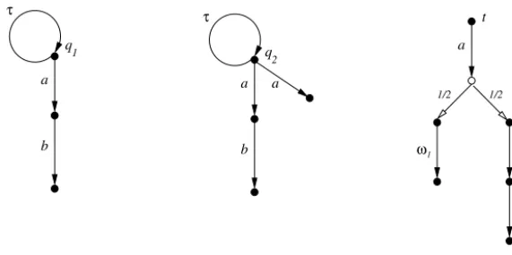
Fig. 1.Two processes with divergence and a test.

powerful than scalar testing that employs only one success action, and likewise reward testing is no more powerful than the special case of reward testing in which all rewards are 1.5

In certain situations it is natural to introduce negative rewards; this is the case, for instance, in the theory of Markov Decision Processes[14]. Intuitively, we could understand negative rewards as costs, while positive rewards are often viewed as benefits or profits. Consider for instance the (nonprobabilistic) processesq1 andq2 ofFig. 1. Herearepresents the action

of making an investment. Assuming that the investment is made by bidding for some commodity, the

τ

-action represents an unsuccessful bid — if this happens one simply tries again. Now b represents the action of reaping the benefits of this investment. Wheresq1 models a process in which making the investment is always followed by an opportunity to reap the

benefits, the process q2 allows, nondeterministically, for the possibility that the investment is unsuccessful, so that adoes

not always lead to a state wherebis enabled. The testt, which will be explained later, allows us to give a negative reward to actiona — its cost — and a positive reward tob.

This leads to the question:if both negative and positive rewards are allowed, how would the original reward-testing semantics change?6 We refer to the more relaxed form of testing, using positive and negative rewards, asreal-reward testingand the original one (from[10], but with probabilistic tests as in[7]) asnonnegative-reward testing.

The power of real-reward testing is illustrated in Fig. 1. The two (nonprobabilistic) processes in the left and central diagrams are equivalent under (probabilistic) may- as well as must-testing; the

τ

-loops in the initial states cause both processes to fail any nontrivial must-test. Yet, if a reward of

−

1 is associated with performing the actiona, and a reward of 2 with the subsequent performance ofb, it turns out that in the first process the net reward is either 0, if the process remains stuck in its initial state, or positive, whereas running the second process may yield a loss. SeeExample 3.8for details of how these rewards are assigned, and how net rewards are associated with the application of tests such ast. This example shows that for processes that may exhibit divergence, real-reward testing is more discriminating than nonnegative-reward testing, or other forms of probabilistic testing. It also illustrates that the extra power is relevant in applications.

As remarked, in [7]we established that for finitary processes the nonnegative-reward must-testing preorder (

nrmust)

coincides with the probabilistic must-testing preorder (

pmust), and likewise for the may-preorders. The main result of

this paper is that restricted to finitary convergent processes, the real-reward must-preorder

rrmust coincides with the

nonnegative-reward must-preorder, i.e. for any finitary convergent processes,

rrmust

Γ

iff

nrmust

Γ.

(1)

Here, as we shall see, convergence is the natural generalisation of the standard concept for nonprobabilistic processes to the probabilistic setting; in particular it rules out the processes ofFig. 1.

There is also a surprisingly simple proof of the fact that for real-reward testing the may- and must-preorders are the inverse of each other, i.e. that for any processes

and

Γ

,

rrmay

Γ

iff

Γ

rrmust

.

(2)

This pleasing symmetry does not hold for the more restrictive nonnegative-reward (or scalar) testing. Moreover, the analogy of(1)for the may-preorder does not hold, i.e.

rrmaydoes not coincide with

nrmay (q.v. the end of Section8).

5 _{In spite of this thereisa difference in power between the notions of testing from[18]and[17], but this is an issue that is entirely orthogonal to} the distinction between scalar testing, reward testing and vector-based testing. In[17]it is the execution of a successactionthat constitutes success, whereas in[1,9,18,10]it is reaching a successstate(even though typically success actions are used to identify those states). In[2, Example 5.3]we showed that state-based testing is (slightly) more powerful than action-based testing. The results presented in[7]about the coincidence of scalar, reward, and vector-based testing preorders pertain to action-based version of each, but in the conclusion it is observed that the same coincidence could be obtained for their state-based versions. In the current paper we stick to state-based testing.

6 _{One might suspect no change at all, for any assignment of rewards from the interval[−1}

(

rrmay

)

−1

Thm.3.7

=

rrmust

Thm.6.4

=

nrmust [

7]

=

pmust [

3]

=

FS

The symbol ‘=’ between two relations means that they coincide for finitary convergent processes.

Fig. 2.The relationship of different testing preorders.

Although it is easy to see that in(1)the former implies the latter, to prove the opposite is far from trivial; see more discussion in Section7. We employ a characterisation of

pmust from[2,3].Failure simulationis a well-known behavioural

preorder for nondeterministic processes [8]; in [2] we showed that it could be adapted to characterise the probabilistic must-testing preorder

pmust, and in[3]this work was generalised from finite to finitary processes. This involved the

gen-eralisation of the standard notion of (weak) derivations in state-based systems[13], to probabilistic processes, i.e. probability distributions. By capitalising on this novel notion of derivation between distributions we can show that the failure simu-lation preorder

FS is contained in

rrmust. Convergence is essential here, even though it is not needed to establish that

FS is contained in

nrmust. Recall that

rrmust is defined usingresolutions; the key to proving this containment, the heart

of the paper, is showing that certain derivations, which we callextreme derivations, are essentially the same asresolutions. Combining this with the results from[7]and[3]mentioned above leads to our required result that

nrmust is included in

rrmust, as far as finitary convergent processes are concerned. Consequently, in this case, all the relations ofFig. 2collapse

into one.

The rest of this paper is organised as follows. We start by recalling notation for probabilistic labelled transition systems. In Section3 we review the resolution-based testing approach and show that the real-reward may-preorder is simply the inverse of the real-reward must-preorder. Moreover, using the example ofFig. 1, we show that in the presence of divergence the inclusion of

rrmust in

nrmust is proper. In Section4 we recall the notions of derivation and the failure simulation

preorder. In Section5we show that resolutions can be seen as certain kinds of derivations. Then in Section6we show for finitary convergent processes that real-reward must-testing coincides with nonnegative-reward must-testing. We explain in Section7why the proof of the coincidence result cannot easily be simplified, and then conclude in Section8.

Besides the related work already mentioned above, many other studies on probabilistic testing and simulation semantics have appeared in the literature. They are reviewed in[6,2]. An extended abstract of the current work has appeared as[5]. All the proofs omitted there are now detailed. Section7is newly added to explain the subtle difference between

rrmust

and

nrmust.

2. Probabilistic processes

A (discrete) probabilitysubdistributionover a set Sis a function

:

S

→ [

0

,

1

]

with

_s∈S

(s)

1; thesupport of such a

is

:= {

s

∈

S

|

(s) >

0

}

, and itsmass

|

|

is

_s∈

(s)

. A subdistribution is a (total, or full)distributionif

|

| =

1. The point distribution s assigns probability 1 to s and 0 to all other elements of S, so that

s

= {

s

}

. With

D

sub

(S)

we denote the set of subdistributions overS, and with

_D

(S)

its subset of full distributions.

Let

{

k

|

k

∈

K

}

be a set of subdistributions, possibly infinite. Then

k∈K

kis the real-valued function inS

→

R

defined by

(

_k∈K

k

)(s)

:=

k∈K

k

(s)

. This is a partial operation on subdistributions because for some states the sum of

k

(s)

might exceed 1. If the index set is finite, say

{

1

..n

}

, we often write

1

+· · ·+

n. Forpa real number from

[

0

,

1

]

we usep

·

to denote the subdistribution given by

(p

·

)(s)

:=

p

·

(s)

. Finally we use

ε

to denote the everywhere-zero subdistribution that thus has empty support. These operations on subdistributions do not readily adapt themselves to distributions; yet if

k∈Kpk

=

1 for some pk

0, and the

k are distributions, then so is

k∈Kpk

·

k.

The expected value

_s∈S

(s)

·

f

(s)

over a subdistribution

of a bounded nonnegative function f to the reals or tuples of them is written Exp

(

f

)

, and the image of a subdistribution

through a function f

:

S

→

T, for some setT, is written

Img_f

()

— the latter is the subdistribution overT given by Img_f

()(t)

:=

_f(s)=t

(s)

for eacht

∈

T.

Definition 2.1.Aprobabilistic labelled transition system(pLTS) is a triple

S,Act,

→

, where

(i) Sis a set of states,

(ii) Actis a set of visible actions,

(iii) relation

→

is a subset of S

×

Actτ

×

D

(S)

.

HereActτ denotesAct

∪ {

τ

}

, where

τ

∈

/

Actis the invisible- or internal action.

A (nonprobabilistic) labelled transition system (LTS) may be viewed as a degenerate pLTS — one in which only point distributions are used. As with LTSs, we writes

−→

α

for

(s,

α

, )

∈ →

, as well ass

−→

α for

∃

:

s

−→

α

ands

→

for

∃

α

:

s

−→

α , withs

−→

α

ands

→

/

representing their negations.

t

−→

α T

Θ

α

∈

/

Act t

p

−→

α

Θ

p

p

−→

τ P

t

p

−→

τ t

[image:4.561.135.386.58.89.2]

t

−→

a T

Θ

p

−→

a P

a

∈

Act t

p

−→

τ

Θ

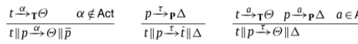
Fig. 3.Synchronous parallel composition between tests and processes.

and statesin

, the support of

, we draw an edge from

tos, labelled with

(s)

. We leave out point-distributions, diverting an incoming edge to the unique state in its support. See e.g.Fig. 4in the next section for some example pLTSs.

In this paper a (probabilistic)processwill simply be a distribution over the state set of a pLTS. A pLTS isdeterministicif for any statesand label

α

there is at most one distribution

withs

−→

α

. It isfinitely branchingif the set

{

|

s

−→

α

,

α

∈

L

}

is finite for all statess; if moreoverSis finite, then the pLTS isfinitary. A subdistribution

over the state setSof an arbitrary pLTS isfinitaryif restricting S to the states reachable from

in the graphical representation of the pLTS yields a finitary sub-pLTS. Similarly, a subdistribution

isfinite if restricting S to the states reachable from

yields a finitary sub-pLTS without loops.

3. Testing probabilistic processes

A testis a finite distribution over the state set of a pLTS having Actτ

∪

Ω

as its set of transition labels, where

Ω

is a

set of fresh successactions, not already inActτ, introduced specifically to report testing outcomes.7 For simplicity we may

assume a fixed pLTS of processes — our results apply to any choice of such a pLTS — and a fixed pLTS of tests. Since the power of testing depends on the expressivity of the pLTS of tests — in particular certain types of tests are necessary for our results — let us just postulate that this pLTS is sufficiently expressive for our purposes — for example that it can be used to interpret all processes from the languagepCSP, as in our previous papers[6,2,3].8

Although we use successactions, they are used merely to mark certain states as success states, namely the sources of transitions labelled by success actions. For this reason we systematically ignore the distributions that can be reached after a success action. We impose two requirements on all states in a pLTS of tests, namely

(A) ift

_−→

ω1 _andt

_−→

ω2 _with

_ω

1

,

ω

2

∈

Ω

then

ω

1

=

ω

2 (uniqueness),

(B) ift

−→

ω with

ω

∈

Ω

andt

−→

α

with

α

∈

Actτ thenu

−→

ω for allu

∈

(no

ω

-disabling).

The first condition says that a success state can have one success identity only, whereas the second condition is a slight weakening of the requirement from[10]that success states must be end states; it allows further progress from an

ω

-success state, for some

ω

∈

Ω

, but

ω

must remain enabled.9

To apply test

Θ

to process

we form a parallel composition

Θ

in whichallvisible actions of

must synchronise with

Θ

. Those synchronisations are immediately renamed into

τ

so that the resulting composition is a process whose only possible actions are the elements of

Ω

τ

:=

Ω

∪ {

τ

}

. Formally, if

P

,

Act,

→

P and

T

,

Act

∪

Ω,

→

T are the pLTSs of processes and tests, then the pLTS of applications of tests to processes is

C

, Ω,

→

, with C

= {

t

p

|

t

∈

T

∧

p

∈

P

}

and

→

the transition relation generated by the rules in Fig. 3. Here if

Θ

∈

D

(

T

)

and

∈

D

(

P

)

, then

Θ

is the distribution given by

(Θ

)(t

p)

:=

Θ(t)

·

(p)

. The resulting pLTS also satisfies (A), (B) above; this would not be the case if we had strengthened (B) to require that success states must be end states.

We will define the result

A

(Θ, )

of applying the test

Θ

to the process

to be a set of testing outcomes, exactly one of which results from each resolution of the choices in

Θ

. Each testing outcomeis an

Ω

-tuple of real numbers in the interval

[

0

,

1

]

, i.e. a functiono

:

Ω

→ [

0

,

1

]

, and its

ω

-componento(

ω

)

, for

ω

∈

Ω

, gives the probability that the resolution in question will reach an

ω

-success state, one in which the success action

ω

is possible.

Due to the presence of nondeterminism in pLTSs, we need a mechanism to reduce a nondeterministic structure into a set of deterministic structures, each of which determines a single possible outcome. Here we adapt the notion ofresolution, defined in[7]for probabilistic automata, to pLTSs.

Definition 3.1 (Resolution).A resolutionof a subdistribution

Φ

∈

D

sub

(S)

in a pLTS

S, Ω,

→

is a triple

R, Λ,

→

R where

R, Ω,

→

R is a deterministic pLTS and

Λ

∈

D

sub

(R)

, such that there exists aresolving function f

:

R

→

Ssatisfying

(i) Imgf

(Λ)

=

Φ

.

(ii) Ifr

−→

α R

Λ

for

α

∈

Ω

τ, then f

(r)

−→

α Imgf

(Λ

)

. (iii) If f

(r)

−→

α for

α

∈

Ω

τ, thenr

−→

α R.

7 _{Forvector-basedtesting we normally takeΩto be countably infinite[17]. This way we have an unbounded supply of success actions for building tests,} of course without obligation to use them all.Scalartesting is obtained by taking|Ω| =1.

8 _{In[3]tests are allowed to be finitary, but if two processes are behaviourally different they can be distinguished by some characteristic tests which are} always finite. Therefore, the results in[3]still hold if tests are required to be finite, as we do here.

[image:5.561.136.408.53.252.2]

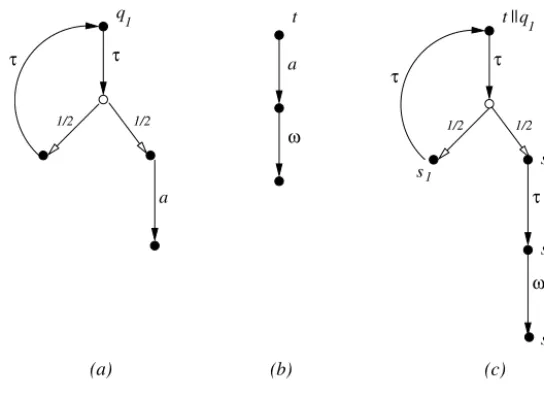
Fig. 4.Testing the processq1.

The reader is referred to Section 2 of [7] for a detailed discussion of the concept of resolution, and the manner in which a resolution represents a run of a process; in particular in a resolution states in S are allowed to be resolved into distributions, and computation steps can be probabilistically interpolated. Our resolutions match the results of applying a scheduler as defined in[16].

We now explain how to associate an outcome with a particular resolution, which in turn will associate a set of outcomes with a subdistribution in a pLTS. Given a deterministic pLTS

R, Ω,

→

R consider the functional

F

:

(R

→ [

0

,

1

]

Ω

)

→

(R

→ [

0

,

1

]

Ω

₎

_{defined by}

F

(

g

)(

r

)(

ω

)

:=

_{1 ifr}

_−→

ω

_,

0 ifr

−→

ω

andr

−→

τ

,

Exp

(

g

)(

ω

)

ifr

−→

ω

andr

−→

τ

.

(3)

We view the unit interval

[

0

,

1

]

ordered in the standard manner as a complete lattice; this induces the structure of a com-plete lattice on the product

[

0

,

1

]

Ω _{and in turn on the set of functions R}

_{→ [}

₀

_,

₁

_]

Ω_{. The functional}

_F

_{is easily seen to be}

monotonic and therefore has a least fixed point, which we denote by

V

R,Ω,→R ; this is abbreviated to

V

when the deter-ministic pLTS in question is understood. Intuitively ExpΛ

(

V

R,Ω,→R

)

is the result of executing the resolution

R, Λ,

→

R starting from the initial distribution

Λ

, a vector of probabilities. FromDefinition 3.1we see that in general a distribution

Φ

gives rise to a nonempty set of resolutions. Collecting all of the possible results of executing them we get

A

(Φ)

=

Exp_Λ

(

V

R,Ω,→R

)

|

R

, Λ,

→

R is a resolution of

Φ

.

(4)

This notation is most often used in calculating the results of applying a test to a process. To emphasise this, we will sometimes use the notation

A

(Θ, )

for

A

(Θ

)

.

Example 3.2. Consider the process q1 depicted in Fig. 4(a). When we apply the test t depicted in Fig. 4(b) to it we get

the processt

q1 depicted inFig. 4(c). This process is already deterministic, hence has essentially only one resolution: itself.

Moreover the outcome Exp_tq

1

(

V

)

=

V

(t

q1

)

associated with it is the least solution of the equation

V

(t

q1

)

=

1

2

·

V

(t

q1

)

+

1

2→−

ω

where→−

ω

:

Ω

→ [

0

,

1

]

is the

Ω

-tuple with→

ω

−

(

ω

)

=

1 and→−

ω

(

ω

)

=

0 for all

ω

=

ω

. In fact this equation has a unique

solution in

[

0

,

1

]

Ω, namely→−

ω

. Thus

A

(t,

q1

)

= {

→−

ω

}

.

2

Example 3.3.Consider the processq2and the application of the testtto it, as outlined inFig. 5. For eachk

1 the process t

q2 has a resolution

Rk

, Λ,

→

Rk such that ExpΛ

(

V

)

=

(

1

−

21k

)

→−

ω

; intuitively it goes around the loop

(k

−

1

)

times before at last taking the right-hand

τ

action. Thus

A

(t,

q2

)

contains

(

1

−

₂1k

)

→−

ω

for everyk

1. But it also contains→−

ω

, because of the resolution which takes the left-hand

τ

-move every time. Thus

A

(t,

q2

)

includes the set

1

−

1 2

−

→

_ω

_,

₁

₋

1

22

−

→

_ω

_{, . . . ,}

₁

₋

1

2k

−

→

_ω

_{, . . . ,}

→−

_ω

_.

As resolutions allow any interpolation between the two

τ

-transitions from states1,

A

(t,

q2

)

is actually the convex closure

[image:6.561.72.468.54.273.2]

Fig. 5.Testing the processq2.

There are two standard methods for comparing two sets of ordered outcomes:

O1

HoO2 if for everyo1

∈

O1there exists someo2

∈

O2such thato1

o2

,

O1

SmO2 if for everyo2

∈

O2there exists someo1

∈

O1such thato1

o2

.

This gives us our definition of the probabilistic may- and must-testing preorders; they are decorated with

·

Ω _{for the}

reper-toire

Ω

of testing actions they employ.

Definition 3.4(Probabilistic testing preorders).

(i)

Ωpmay

Γ

if for every

Ω

-test

Θ

,

A

(Θ, )

Ho

A

(Θ, Γ )

,

(ii)

Ω_pmust

Γ

if for every

Ω

-test

Θ

,

A

(Θ, )

Sm

A

(Θ, Γ )

.

These preorders are abbreviated to

pmay

Γ

and

pmust

Γ

when

|

Ω

|=

1.

In[7]we established that for finitary processes

Ω

pmay coincides with

pmayand

Ωpmustwith

pmustfor any choice of

Ω

.

We also defined the reward-testing preorders in terms of the mechanism set up so far. The idea is to associate with each success action

ω

∈

Ω

a reward, which is a nonnegative number in the unit interval

[

0

,

1

]

; and then a run of a probabilistic process in parallel with a test yields an expected reward accumulated by those states which can enable success actions. A reward tuple h

∈ [

0

,

1

]

Ω _{is used to assign reward h(}

_ω

₎

_{to success action}

_ω

_{, for each}

_ω

_∈

_Ω

_{. Due to the presence of}

nondeterminism, the application of a test

Θ

to a process

produces a set of expected rewards. Two sets of rewards can be compared by examining their suprema/infima; this gives us two methods of testing called reward may/must testing. In [7] all rewards are required to be nonnegative, so we refer to that approach of testing as nonnegative-reward testing. If we also allow negative rewards, which intuitively can be understood as costs, then we obtain an approach of testing calledreal-reward testing. Technically, we simply let reward tupleshrange over the set

[−

1

,

1

]

Ω_{. Ifo}

_{∈ [}

₀

_,

₁

_]

Ω_{, we use the}

dot-producth

·

o

=

_ω∈Ωh(

ω

)

·

o(

ω

)

. It can apply to a set O

⊆ [

0

,

1

]

Ω so thath

·

O

= {

h

·

o

|

o

∈

O

}

. LetA

⊆ [−

1

,

1

]

. We use the notation

A for the supremum of set A, and

A for the infimum.

Definition 3.5(Reward-testing preorders).

(i)

Ωnrmay

Γ

if for every

Ω

-test

Θ

and nonnegative-reward tupleh

∈ [

0

,

1

]

Ω,

h

·

A

(Θ, )

h

·

A

(Θ, Γ ),

(iii)

Ωrrmay

Γ

if for every

Ω

-test

Θ

and real-reward tupleh

∈ [−

1

,

1

]

Ω,

h

·

A

(Θ, )

h

·

A

(Θ, Γ ),

(iv)

Ω

rrmust

Γ

if for every

Ω

-test

Θ

and real-reward tupleh

∈ [−

1

,

1

]

Ω,

h

·

A

(Θ, )

h

·

A

(Θ, Γ ).

This time we drop the superscript

Ω

iff

Ω

is countably infinite.

It is shown in Corollary 1 of[7]that nonnegative-reward testing is equally powerful as probabilistic testing.

Theorem 3.6.(See[7].) For any finitary processes

and

Γ

,

(i)

nrmay

Γ

if and only if

pmay

Γ

,

(ii)

nrmust

Γ

if and only if

pmust

Γ

.

In this paper we focus on the real-reward testing preorders

rrmay and

rrmust, by comparing them with the

nonnegative-reward testing preorders

nrmay and

nrmust. Although these two nonnegative-reward testing preorders are

in general incomparable, we have for the real-reward testing preorders:

Theorem 3.7.For any processes

and

Γ

, it holds that

rrmay

Γ

if and only if

Γ

rrmust

.

Proof. We first notice that for any nonempty setA

⊆ [

0

,

1

]

Ω _{and any reward tupleh}

_{∈ [−}

₁

_,

₁

_]

Ω_,

h

·

A

= −

(

−

h

)

·

A

,

(5)

where

−

his the negation ofh, i.e.

(

−

h)(

ω

)

= −

(h(

ω

))

for any

ω

∈

Ω

. We consider the “if” direction; the “only if” direction is similar. Let

Θ

be any

Ω

-test andhbe any real-reward tuple in

[−

1

,

1

]

Ω_{. Clearly,}

₋

_{his also a real-reward tuple. Suppose}

Γ

rrmust

, then

(

−

h

)

·

A

(Θ, Γ )

(

−

h

)

·

A

(Θ, ).

(6)

Therefore, we can infer that

h

·

A

(Θ, )

= −

(

−

h

)

·

A

(Θ, )

by(5)

−

(

−

h

)

·

A

(Θ, Γ )

by(6)

=

h

·

A

(Θ, Γ )

by(5).

2

Our next task is to compare

rrmust with

nrmust. The former is included in the latter, which directly follows from Definition 3.5. Surprisingly, it turns out that for finitary convergent processes the latter is also included in the former, thus establishing that the two preorders are in fact the same. The rest of the paper is devoted to proving this result. However, we first show that this result does not extend to divergent processes.

Example 3.8. Consider the processesq1 andq2 depicted inFig. 1. Using the characterisations of

pmay and

pmust in[3],

it is easy to see that these processes cannot be distinguished by probabilistic may- and must-testing, and hence not by nonnegative-reward testing either. However, let t be the test in the right diagram ofFig. 1 that first synchronises on the actiona, and then with probability 1₂ reaches a state in which a reward of

−

2 is allocated, and with the remaining prob-ability 1₂ synchronises with the actionb and reaches a state that yields a reward of 4. Thus the test employs two success actions

ω

1 and

ω

2, and we use the reward tuplehwithh(

ω

1

)

= −

2 andh(

ω

2

)

=

4. Then the resolution of q1 that does

not involve the

τ

-loop contributes the value

−

2

·

1₂

+

4

·

1₂

= −

1

+

2

=

1 to the set h

·

A

(t,

q1

)

, whereas the resolution

that only involves the

τ

-loop contributes the value 0. Due to interpolation,h

·

A

(t,

q1

)

is in fact the entire interval

[

0

,

1

]

.

On the other hand, the resolution corresponding to thea-branch ofq2 contributes the value

−

1 andh

·

A

(t,

q2

)

= [−

1

,

1

]

.

4. Failure simulations

In this section we explain the characterisation of probabilistic testing from[2,3]; it depends on a generalisation of failure simulations [8] to the probabilistic setting. The key ingredient is that of weak derivations for distributions. To deal with infinite (but finitary) processes, we need to employ the weak derivations of [3]rather than those of[2].

In a pLTS actions are performed only by states, in that actions are given by relations from states to distributions. But processes in general correspond to distributions over states, so in order to define what it means for a process to perform an action, we need toliftthese relations so that they also apply to distributions. In fact we will find it convenient to lift them to subdistributions.

Definition 4.1.Let

(S,

L,

→

)

be a pLTS and

R

⊆

S

×

D

sub

(S)

be a relation from states to subdistributions. Then

R

⊆

D

sub

(S)

×

D

sub

(S)

is the smallest relation that satisfies:

(i) s

R

impliess

R

, and

(ii) (Linearity)

Γ

i

R

ifori

∈

Iimplies

(

i∈Ipi

·

Γ

i

)

R

(

i∈Ipi

·

i

)

for any pi

∈ [

0

,

1

]

(i

∈

I) with

i∈Ipi

1, where I is a countable set.

An application of this notion is when the relation is

−→

α for

α

∈

Actτ; in that case we also write

−→

α for

→

α. Thus,

as source of a relation

−→

α we now also allow distributions, and even subdistributions. A subtlety of this approach is that for any action

α

, we have

ε

−→

α

ε

simply by taking I

= ∅

or

_i∈Ipi

=

0 inDefinition 4.1. That turns out to make

ε

especially useful for modelling the “chaotic” aspects of divergence in [3], in particular that in the must-case a divergent process can mimic any other.

Definition 4.1is very similar to our previous definition in[2], although there it applied only to (full) distributions:

Lemma 4.2.

Γ

R

if and only if

(i)

Γ

=

i∈Ipi

·

si, where I is an index set and

i∈Ipi

1, (ii) for each i

∈

I there is a subdistribution

isuch that si

R

i, (iii)

=

_i∈Ipi

·

i.

Proof. Straightforward.

2

An important point here is that a single state can be split into several pieces: that is, the decomposition of

Γ

into

i∈Ipi

·

siis not unique.

Definition 4.3(Weak derivation).Suppose we have subdistributions

,

→_k

,

×_k, fork

0, with the following properties:

=

→₀

+

×₀

,

→₀

−→

τ

→₁

+

×₁

,

..

.

_k→

−→

τ

→_k+1

+

_k×₊₁

.

..

.

Then we call

:=

∞_k=0

×_k aweak derivativeof

, and write

=⇒

to mean that

can make aweak derivationto its derivative

.

There is always at least one weak derivative of any subdistribution (the subdistribution itself) and there can be many.

Proposition 4.4(Transitivity, linearity and decomposition of weak derivations). (See[4].)

(i) If

=⇒

and

=⇒

then

=⇒

. Let pi

∈ [

0

,

1

]

for i

∈

I with

i∈Ipi

1. (ii) If

i

=⇒

ifor all i

∈

I then

i∈Ipi

·

i

=⇒

i∈Ipi

·

i. (iii) If

_i∈Ipi

·

i

=⇒

then

=

i∈Ipi

·

ifor subdistributions

isuch that

i

=⇒

ifor all i

∈

I.

Definition 4.5.Let

and its variants

,

pre

,

post be subdistributions in a pLTS

S,Act,

→

.

•

Fora

∈

Actwrite

=⇒

a

whenever

=⇒

pre

−→

a

post

=⇒

, for some

pre and

post. Extend this toActτ by allowing

as a special case that

=⇒

τ is simply

=⇒

, i.e. including identity (rather than requiring at least one

−→

τ ).

•

ForA

⊆

Actands

∈

Swrites

−→

A ifs

−→

α

for every

α

∈

A

∪ {

τ

}

; write

−→

A ifs

−→

A for everys

∈

.

•

More generally write

=⇒

−→

A if

=⇒

prefor some

presuch that

pre

−→

A .

Definition 4.6(Failure simulation preorder).Define

FSto be the largest relation in S

×

D

sub

(S)

such that ifs

FS

then

(i) whenevers

=⇒

α

Γ

, for

α

∈

Actτ, then there is a

∈

D

sub

(S)

with

=⇒

α

and

Γ

FS

, (ii) and whenevers

=⇒

−→

A then

=⇒

−→

A .

Any relation

R

⊆

S

×

D

sub

(S)

that satisfies the two clauses above is called afailure simulation. The failure simulation preorder

FS

⊆

D

sub

(S)

×

D

sub

(S)

is defined by letting

FS

Γ

whenever there is a

with

=⇒

and

Γ

FS

.

Note that the simulating process,

, occurs at the right of

FS, but at the left of

FS. The following lemma will bee needed in Section6.

Lemma 4.7.If

Γ

FS

and

Γ

=⇒

Γ

then there is a matching transition

=⇒

such that

Γ

FS

.

Proof.

Γ

FS

implies byLemma 4.2that

Γ

=

i∈I

pi

·

si

,

si

FS

i

,

=

i∈I pi

·

i

.

By Proposition 4.4(iii) there are

Γ

_i

∈

D

sub

(S)

fori

∈

I with si

=⇒

Γ

i and

Γ

=

pi∈Ipi

·

Γ

i. For eachi

∈

I we infer from si

FS

i andsi

=⇒

Γ

ithat there is a

i

∈

D

sub

(S)

with

i

=⇒

iand

Γ

i

FS

. Let

:=

i∈Ipi

·

i. ThenDefinition 4.1(2) andProposition 4.4(ii) yield

Γ

FS

and

=⇒

.

2

The failure simulation preorder is preserved under parallel composition with a test and it is sound and complete for probabilistic must-testing of finitary processes.

Theorem 4.8.(See[3].) For finitary processes

and

Γ

,

(i) if

FS

Γ

then for any

Ω-test

Θ

,

Θ

FS

Θ

Γ

, (ii)

FS

Γ

if and only if

pmust

Γ

.

5. From derivations to resolutions

In this section we explain how resolutions, on which the definitions of the testing preorders inDefinitions 3.4 and 3.5

are based, can be seen as certain kinds of derivations.

Definition 5.1(Extreme derivatives).A statesin a pLTS is calledstableifs

−→

τ

, and a subdistribution

is calledstableif every state in its support is stable. We write

=⇒

whenever

=⇒

and

is stable, and call

anextremederivative of

.

Referring toDefinition 4.3, we see this means that in the extreme derivation of

from

at every stage a state must move on if it can, so that every stopping component can contain only states whichmuststop: fors

∈

→_k

+

×_k

we have s

∈

×_k

ifand now alsoonly ifs

−→

τ .

Lemma 5.2(Existence and uniqueness of extreme derivatives).

(i) For every subdistribution

there exists some(stable)

such that

=⇒

. (ii) In a deterministic pLTS if

=⇒

and

=⇒

then

=

.

Proof. We construct a derivation as in Definition 4.3of a stable

by defining the components

k

,

×k and

→k using induction onk. Let us assume that the subdistribution

k has been defined; in the base casek

=

0 this is simply

. The decomposition of this

k into the components

×_k and

→_k is carried out by defining the former to be precisely those states which must stop, i.e. thosesfor whichs

−→

τ

. Formally

×_k is determined by:

×_k

(

s

)

=

k

(

s

)

ifs

−→

τ

,

Then

→_k is given by theremainderof

k, namely those states which can perform a

τ

action:

_k→

(

s

)

=

k

(

s

)

ifs

−→

τ

,

0 otherwise

.

Note that these definitions divide the support of

k into two disjoints sets, namely the support of

k× and the support of

_k→. Moreover by construction we know that

_k→

−→

τ

Θ

for some

Θ

; we let

k+1 be an arbitrary such

Θ

.

This completes our construction of an extreme derivative as inDefinition 4.3and so we have established (i).

For (ii) we observe that in a deterministic pLTS the above choice of

k+1 is unique, so that the whole derivative

con-struction becomes unique.

2

Subdistributions are essential in the definition of extreme derivations. Consider a statet that has only one transition, a self

τ

-loopt

−→

τ t. Then it diverges and it has a unique extreme derivative

ε

, the empty subdistribution. More generally, suppose a subdistribution

diverges, that is there is an infinite sequence of internal transitions

−→

τ

1

−→ · · ·

τ

−→

τ

k

−→ · · ·

τ . Then one extreme derivative of

is

ε

, but it may have others.

In the extreme derivative

=⇒

, the subdistribution

may be viewed as a final result of an execution starting in

and dynamically resolving nondeterministic choices as the execution proceeds. We can tabulate the outcome of this execution in the following manner:

Definition 5.3 (Outcomes). The outcome $

Φ

∈ [

0

,

1

]

Ω _{of a stable subdistribution}

_Φ

_{is given by $}

_Φ(

_ω

₎

₌

_{

_Φ(s)

_|

_s

_∈

Φ

,

s

−→}

ω . For any distribution

Φ

we write

V

(Φ)

for the set of possible outcomes

{

$

Φ

|

Φ

=⇒

Φ

}

via extreme derivatives.

Letpi

∈ [

0

,

1

]

fori

∈

Iwith

i∈Ipi

1, and let

i

, Φ

i, fori

∈

I, be subdistributions. We use

i∈Ipi

·

V

(

i

)

as shorthand for

{

_i∈Ipi

·

ν

i

|

ν

i

∈

V

(

i

)

}

. By construction, $

i∈Ipi

·

Φ

i

=

i∈Ipi

·

$

Φ

i. Using this, we establish the linearity of

V

:

Lemma 5.4.Let pi

∈ [

0

,

1

]

for i

∈

I with

i∈Ipi

1. Then

V

(

i∈Ipi

·

i

)

=

i∈Ipi

·

V

(

i

).

Proof. Suppose

ν

∈

V

(

i∈Ipi

·

i

)

. Then

ν

=

$

Φ

for some stable

Φ

with

i∈Ipi

·

i

=⇒

Φ

. ByProposition 4.4(iii)

Φ

can be written as

_i∈Ipi

·

Φ

i for subdistributions

Φ

i such that

i

=⇒

Φ

i for all i

∈

I; moreover, the

Φ

i must be stable. Hence

ν

i

:=

$

Φ

i

∈

V

(

i

)

and thus

ν

=

i∈Ipi

·

ν

i

∈

i∈Ipi

·

V

(

i

)

.

Conversely, suppose

ν

∈

_i∈Ipi

·

V

(

i

)

, i.e.,

ν

=

i∈Ipi

·

ν

iwith

ν

i

∈

V

(

i

)

. Then for alli

∈

Ithere are stable subdistri-butions

Φ

iwith

ν

i

:=

$

Φ

iand

i

=⇒

Φ

i. So

i∈Ipi

·

i

=⇒

i∈Ipi

·

Φ

i byProposition 4.4(ii). Moreover

i∈Ipi

·

Φ

i is stable and

ν

=

i∈Ipi

·

ν

i

=

$

i∈Ipi

·

Φ

i

∈

V

(

i∈Ipi

·

i

)

.

2

The following two examples illustrate that this manner of calculating outcomes often gives the same result as when resolutions are used.

Example 5.5. (RevisitingExample 3.2.) The pLTS in Fig. 4(c) is deterministic and therefore from part (ii) of Lemma 5.2it follows thatt

q1 has a unique extreme derivative

Λ

. Moreover

Λ

can be calculated to be

k1₂1k

·

s3, which simplifies to the distribution s3. Therefore, since $s3

=

→−

ω

, it follows that

V

(t

q1

)

= {

→−

ω

}

. This is exactly the same result as obtained in Example 3.2, using resolutions.

2

Example 5.6. (RevisitingExample 3.3.) The application of the testt to processesq2 is outlined in Fig. 5(c). Consider any

extreme derivative

froms0

=

t

q2. Using the notation ofDefinition 4.3, it is clear that

×0 and

→0 must be

ε

ands0

respectively. Similarly,

×₁ and

→₁ must be

ε

ands1 respectively. Buts1 is a nondeterministic state, having two possible

transitions:

(i) s1

−→

τ

Λ

0where

Λ

0 has support

{

s0

,

s2

}

and assigns each of them the weight 1₂,

(ii) s1

−→

τ

Λ

1where

Λ

1 has the support

{

s3

,

s4

}

, again dividing the mass equally among them.

So there are many possibilities for

2; fromDefinition 4.3one sees that in fact

2 can be of the form

p

·

Λ

0

+

(

1

−

p

)

·

Λ

1 (7)

for any choice of p

∈ [

0

,

1

]

.

Let us consider one possibility, an extreme one where pis chosen to be 0; only the transition (ii) above is used. Here

→₂ is the subdistribution 1₂s4, and

→_k

=

ε

wheneverk

>

2. A simple calculation shows that in this case the extreme

derivative generated is

Λ

e₁

=

1₂s3

+

1₂s6which implies that 1₂→−

ω

∈

V

(t

q2

)

.

Another possibility for

2 is

Λ

0, corresponding to p

=

1 in (7)above. Continuing this derivation leads to

3 being 1

2

·

s1

+

1

2

·

s5; thus

×3

=

1

2

·

s5 and

→3

=

1

the nondeterministic states1, by choosing some arbitraryp

∈ [

0

,

1

]

in(7). Suppose we choose p

=

1 every time, completely

ignoring transition (ii) above. Then the extreme derivative generated is

Λ

e₀

=

k1

1 2k

·

s5

,

which simplifies to the distributions5. This in turn means that→−

ω

∈

V

(t

q2

)

.

We have seen two possible derivations of extreme derivatives from s0. But there are many others. In general whenever

_k→is of the formq

·

s1 we have to resolve the nondeterminism by choosing ap

∈ [

0

,

1

]

in(7)above; moreover each such

choice is independent. It turns out that every extreme derivative

ofs0is of the formq

·

Λ

0e

+

(

1

−

q)

·

Λ

e1 for some choice

ofq

∈ [

0

,

1

]

, which implies that

V

(t

q2

)

is the convex closure of the set

{

12→−

ω

,

→−

ω

}

.

Again this is similar to the results obtained using resolutions, inExample 3.3.

2

Unfortunately there is not an exact agreement between using resolutions and extreme derivations, as the next example shows.

Example 5.7. Let pbe a process that first does ana-action, to the point distributionq, and then diverges, via the

τ

-loop q

−→

τ q. Lett be the test used inExamples 3.2 and 3.3. It is easy to see that the distribution p

t has a unique resolution, with expected outcome→−

ω

; thus

A

(t,

p)

= {

→−

ω

}

.

It turns out thatt

palso has a unique extreme derivative; unfortunately this turns out to be

ε

. Since $

ε

=

0 this means that

V

(t

p)

=

→−0; so in this case, which is actually nonprobabilistic, there is a difference between the use of resolutions and extreme derivations.

2

To rectify this anomaly, we restrict our attention to a subset of pLTSs.

Definition 5.8(

ω

-respecting).A pLTS

S, Ω,

→

is said to be

ω

-respectingwhen it satisfies the uniqueness requirement (A) from p.4, ands

−→

ω , for any

ω

∈

Ω

, impliess

−→

τ .

It is straightforward to modify the pLTS of applications of tests to processes into one that it is

ω

-respecting, namely by removing all transitions s

−→

τ

for states s withs

−→

ω ; we call thispruning. We denote the result of pruning the pLTS

S, Ω,

→

by

S, Ω,

[→]

, and the distribution

Φ

in this pruned pLTS by

[

Φ

]

.

Example 5.9.(RevisitingExample 5.7.) Let p,q andt be as in Example 5.7. As we have already seen, t

p has the unique derivative

ε

. But by pruning it we obtain a different extreme derivative. If we denote the state reachable from t with the outgoing

ω

-transition, inFig. 5(c), as

ω

also, then

[

t

p

]

has the unique extreme derivative

[

ω

q

]

. Since $

[

ω

q

] =

→−

ω

, we obtain

V

(

[

t

p

]

)

= {

→−

ω

}

; this is exactly the result obtained using resolutions.

2

Note that pruning has no effect onExamples 5.5 and 5.6, as the pLTSs concerned are already

ω

-respecting. It also has no effect on the closure of the failure simulation preorder under parallel composition:

Lemma 5.10.(See[4].) For finitary processes

and

Γ

, if

FS

Γ

then for any

Ω-test

Θ

,

[

Θ

]

FS

[

Θ

Γ

]

.

In the remainder of this section we show that, at least in

ω

-respecting pLTSs, using resolutions to calculate outcomes, as used in the definition of testing (Definitions 3.4 and 3.5), leads to the same results as using extreme derivations. In the former a set of deterministic structures are associated with a distribution, while in the latter nondeterministic choices are resolved dynamically as the derivation proceeds. We start by showing that resolution-based testing is insensitive to pruning. Let

A

p

(Φ)

denote the set of vectors

Exp_Λ

(

V

R,Ω,→R

)

R

, Λ,

→

R is a resolution of

[

Φ

]

.

Proposition 5.11.For any distribution

Φ

in a pLTS

S, Ω,

→

we have that

A

p

_(Φ)

₌

_A

_(Φ).

Proof. “

⊇

”: Let

R, Λ,

→

R be a resolution of

Φ

. Then, followingDefinition 3.1,

R,

[

Λ

]

,

[→

R

]

is a resolution of

[

Φ

]

and, by(3), Exp_[Λ]

(

V

R,Ω,[→R]

)

=

ExpΛ

(

V

R,Ω,→R

)

.

“

⊆

”: Let

R, Λ,

→

R be a resolution of

[

Φ

]

with resolving function f. We construct a resolution

R

, Λ,

→

_R of

Φ

as a random extension of

R, Λ,

→

R . For every pair

(s,

α

)

∈

S

×

Ω

τ withs

−→

α pick a distribution

Ψ

(s,α)

∈

D

(S)

such that