Proceedings of the 2nd Workshop on Computational Approaches to Subjectivity and Sentiment Analysis, ACL-HLT 2011, pages 44–52,
Developing Robust Models for Favourability Analysis
Daoud Clarke Peter Lane
School of Computer Science University of Hertfordshire
Hatfield, UK
[email protected] [email protected]
Paul Hender
Metrica London, UK
Abstract
Locating documents carrying positive or neg-ative favourability is an important application within media analysis. This paper presents some empirical results on the challenges fac-ing a machine-learnfac-ing approach to this kind of opinion mining. Some of the challenges in-clude: the often considerable imbalance in the distribution of positive and negative samples; changes in the documents over time; and ef-fective training and quantification procedures for reporting results. This paper begins with three datasets generated by a media-analysis company, classifying documents in two ways: detecting the presence of favourability, and as-sessing negative vs. positive favourability. We then evaluate a machine-learning approach to automate the classification process. We ex-plore the effect of using five different types of features, the robustness of the models when tested on data taken from a later time period, and the effect of balancing the input data by undersampling. We find varying choices for the optimum classifier, feature set and training strategy depending on the task and dataset.
1 Introduction
Media analysis is a discipline closely related to con-tent analysis (Krippendorff, 2004), with an emphasis on analysing content with respect to:
Favourability how favourable an article is with respect to an entity. This will typically be on a five point scale: very negative, negative, neutral, positive or very positive.
Key messages topics or areas that a client is inter-ested in. This allows the client to gain feedback on the success of particular public relations campaigns, for example.
Media analysis has traditionally been done manu-ally, however the explosion of content on the world-wide web, in particular social media, has led to the introduction of automatic techniques for performing media analysis, e.g. Tatzl and Waldhauser (2010).
In this paper, we discuss our recent findings in ap-plying machine learning techniques to favourability analysis. The work is part of a two-year collabo-ration between Gorkana Group, which includes one of the foremost media analysis companies, Metrica, and the University of Hertfordshire. The goal is to develop ways of automating media analysis, espe-cially for social media. The data used are from tra-ditional media (newspapers and magazines) since at the time of starting the experiment there was more manually analysed data available. We discuss the typical problems that arise in this kind of text min-ing, and the practical results we have found.
The documents are supplied by Durrants, the me-dia monitoring company within the Gorkana Group, and consist of text from newspaper and magazine articles in electronic form. Each document is anal-ysed by trained human analysts, given scores for favourability, as well as other characteristics which the client has requested. This dataset is used to pro-vide feedback to the clients about how they are por-trayed in the media, and is summarised by Metrica for clients’ monthly reports.
Favourability analysis is very closely related to sentiment analysis, with the following distinction:
sentiment analysis generally focuses on a (subjec-tive) sentiment implying an opinion of the author, for example:1
(1) Microsoft is the greattteesssst at EVERY-THING
expresses the author’s opinion (which others may not share) whereas favourability analysis, whilst also taking into account sentiment, also measures favourable objective mentions of entities. For ex-ample:2
(2) Halloween Eve Was The Biggest Instagram Day Ever, Doubling Its Traffic
is an objective statement (no one can doubt that the traffic doubled) that is favourable with respect to the organisation, Instagram. Since the task is so simi-lar to that of sentiment analysis, we hypothesise that similar techniques will be useful.
The contributions of this paper are as follows: (1) whilst automated sentiment analysis has received a lot of attention in the academic literature, favourabil-ity analysis has so far not benefited from an in-depth analysis. (2) We provide results on a wide variety of different classifiers, whereas previous work on sen-timent analysis typically considers at most two or three different classifiers. (3) We discuss the prob-lem of imbalanced data, looking at how this impacts on the training and evaluation techniques. (4) We show that both attribute selection and balancing the classifier’s training set can improve performance.
2 Background
There is a very large body of literature on both sen-timent analysis and machine learning; for space rea-sons, we will mention only a small sample.
2.1 Favourability Analysis
The most closely related task to ours is arguably opinion mining, i.e. determining sentiment with re-spect to a particular target. Balahur et al. (2010) examine this task for newspaper articles. They show that separating out the objective favourabil-ity from the expressed sentiment led to an increase
1
Actually, this is an ironic comment on a blog post at TechCrunch.
2
A headline from TechCrunch
in inter-annotator agreement, which they report as 81%, after implementing improvements to the pro-cess. Melville et al. (2009) report on an automated system for opinion mining applied to blogs, which achieves between 64% and 91% accuracy, depend-ing on the domain, while Godbole et al. (2007) de-scribe a system applied to news and blogs.
Pang et al. (2002) introduced machine learning to perform sentiment analysis. They used na¨ıve bayes, support vector machines (SVMs) and maximum en-tropy on the movie review domain, and report ac-curacies between 77% and 83% depending on the feature set, which included unigrams, bigrams, and part-of-speech tagged unigrams. More recent work along these lines is described in (Pang and Lee, 2008; Prabowo and Thelwall, 2009).
One approach to sentiment analysis is to build up a lexicon of sentiment carrying words. Turney (2002) described a way to automatically build such a lexicon based on looking at co-occurrences of words with other words whose sentiment is known. This idea was extended by Gamon et al. (2005) who also considered the lack of co-occurrence as useful infor-mation.
Koppel and Schler (2006) show that it is impor-tant to distinguish the two tasks of determining neu-tral from non-neuneu-tral sentiment, and positive versus negative sentiment, and that doing so can signifi-cantly improve the accuracy of automated systems.
2.2 Machine Learning Approaches
Document classification is an ideal domain for ma-chine learning, because the raw data, the text, are easily manipulated, and often large amounts of text can be obtained, making the problems amenable to statistical analysis.
A classification model is essentially a mapping, from a document described as a set of feature values to a class label. In most cases, this class label is a simple yes-no choice, such as whether the document is favourable or not. In the experimental section of this paper we describe results from applying a range of different classification algorithms.
2.2.1 Features
Useful features for constructing classification models from text documents include sets of uni-grams, bigrams or triuni-grams, dependency relation-ships or selected words: we review these features in the next section. From a machine-learning perspec-tive, it is useful for the features to include only rele-vant information, and also to be independent of each other. This feature-selection problem has been tack-led by several authors in different ways, e.g. (Blum and Langley, 1997; Forman, 2003; Green et al., 2010; Mladeni´c, 1998; Rogati and Yang, 2002). In our experiments, we evaluate a technique to reduce the number of features using attribute selection.
Alternative approaches to understanding the sen-timent of text attempt to go beyond the simple la-belling of the presence of a word. Some authors have described experiments augmenting the above feature sets with additional information. Mullen and Collier (2004), for example, uses WordNet to add in-formation about words found within text, and conse-quently reports improved classification performance in a sentiment analysis task.
2.3 Imbalanced Data
Our datasets, as is usual in many real-world applica-tions, present varying degrees of imbalance between the two classes. Imbalanced data must be dealt with at two parts of the process: during training, to ensure the model is capable of working with both classes, and in evaluation, to ensure a model with the best performance is selected for use on novel data. These two elements are often treated together, but need to be considered separately. In particular, the appropri-ate training method to handle imbalanced data can vary between algorithm and domain.
First considering evaluation, the standard mea-sure of accuracy (proportion of correctly classified examples) is inappropriate if 90% of the documents are within one class. A simple ZeroR classifier (se-lecting the majority class) will score highly, but it will never get any examples of the minority class correct. A better evaluation technique uses a combi-nation of the separate accuracy measures on the two classes (a1anda2), whereaidenotes the proportion of instances from classithat were judged correctly. For example, the geometric mean, as proposed by
Kubat et al. (1998), computes√a1×a2. This has the property that it strongly penalises poor perfor-mance in any one class: if eithera1ora2is zero then the geometric mean will be zero. This characteristic is important for our purposes, since it is “easy” to get high accuracy on the majority class, the measure will favour classifiers that perform well on the mi-nority class without significant loss of accuracy in the majority class. In addition, the geometric mean does not give preference to any one class, unlike, for example, the F-measure. Measures such as the av-erage precision and recall, or F-measure, may also prove useful, especially if preference is being given to one class.
Second considering the training process. An im-balanced training set can lead to bias in the construc-tion of a machine-learning model. Such effects are well-known in the literature, and various approaches have been proposed to address this problem, such as balancing the training set using under or over sam-pling, and altering the weighting of the classifier based on the proportion of the expected class. In our experiments we used undersampling (where a ran-dom sample is taken from the majority class to bal-ance the size of the minority class); this technique has the disadvantage of discarding training data. In contrast, the SMOTE (Chawla et al., 2004) algo-rithm is a technique for creating new instances of the minority class, to balance the number in the major-ity class. We also used geometric-mean as the eval-uation measure for algorithms such as SVMs, when selecting parameters.
3 Our Approach
3.1 Description of Data
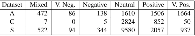
Dataset Mixed V. Neg. Negative Neutral Positive V. Pos.
A 472 86 138 1610 1506 1664
C 7 0 5 2824 852 50
[image:4.612.152.464.71.129.2]S 522 94 344 9580 2057 937
Table 1: Number of documents in each class for the datasets A, C and S.
Dataset Neutral Non-neutral
A 1610 3866
C 2824 914
[image:4.612.108.264.165.223.2]S 9580 3954
Table 2: Class distributions for pseudo-subjectivity task
f >0andu >0: mixed
f = 0andu >1: very negative
f = 0andu = 1: negative
f = 0andu = 0: neutral
f = 1andu = 0: positive
f >1andu = 0: very positive
Table 1 shows the number of documents in each category for three datasets A, C and S, which are anonymised to protect Metrica’s clients’ privacy. A and S are datasets for high-tech companies, whereas C is for a charity. This is reflected in the low oc-curence of negative favourability with dataset C. Datasets A and C contain only articles that are rele-vant to the client, whereas S contains articles for the client’s competitors. We only make use of favoura-bility judgments with respect to the client, however, so those that are irrelevant to the client we simply treat as neutral. This explains the overwhelming bias towards neutral sentiment in dataset S.
In our experiments, we consider only those doc-uments which have been manually analysed and for which the raw text is available. Duplicates were re-moved from the dataset. Duplicate detection was performed using a modified version of Ferret (Lane et al., 2006) which compares occurrences of charac-ter trigrams between documents. We considered two documents to be duplicates if they had a similarity score higher than 0.75.
This paper describes experiments for two tasks:
Pseudo-subjectivity — detecting the presence or
ab-sence of favourability. This is thus a two-class prob-lem with neutral documents in one class, and all other documents in the other.
Dataset Positive Negative
A 3170 224
C 902 5
S 2994 438
Table 3: Class distributions for pseudo-sentiment task
Pseudo-sentiment — distinguishing between
docu-ments with generally positive and negative favoura-bility. In our experiments, we treat this as a two class problem, with negative and very negative docu-ments in one class and positive and very positive documents in the other (ignoring mixed sentiment).
3.2 Method
We follow a similar approach to Pang et al. (2002): we generate features from the article text, and train a classifier using the manually analysed data.
We sorted the documents by time, and then se-lected the earliest two thirds as a training set, and kept the remainder as a held out test set. This al-lows us to get an idea of how the system will per-form when it is in use, since the system will neces-sarily be trained on documents from an earlier time period. We performed cross validation on the ran-domised training set, giving us an upper bound on the performance of the system, and we also mea-sured the accuracy of every system on the held out dataset. We hypothesised that new topics would be discussed in the later time frame, and thus the accu-racy would be lower, since the system would not be trained on data for these topics.
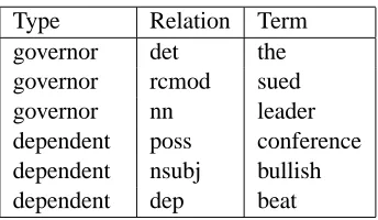
[image:4.612.355.496.166.222.2]Type Relation Term
governor det the
governor rcmod sued
governor nn leader
dependent poss conference
dependent nsubj bullish
[image:5.612.100.272.69.169.2]dependent dep beat
Table 4: Example dependency relations extracted from the data. “Type” indicates whether the term referring to the organisation is the governor or the dependent in the expression.
3.2.1 Features for documents
We used five types of features:
Unigrams, bigrams and trigrams: produced using
the WEKA tokenizer with the standard settings.3 EntityWords: unigrams of words occurring within
a sentence containing a mention of the organisation in question. Mentions of the organisation were de-tected using manually constructed regular expres-sions, based on datasets for organisations collected elsewhere in the company. Sentence boundary de-tection was performed using an OpenNLP4tool.
Dependencies: we extract dependencies using the
Stanford dependency parser. For the purpose of this experiment, we only considered dependencies directly connecting the term relating to the organ-isation. Table 4 gives example dependencies ex-tracted from the data. For example, the phrase “. . . prompted [organisation name] to be bullish. . . ” led to the extraction of the term bullish, where the organisation name is the subject of the verb and the organisation name is a dependent of the verb bullish. For each dependency, all this information is com-bined into a single feature.
3.3 Classification Algorithms
We used the following classifiers in our experiments: na¨ıve Bayes, Support Vector Machines (SVMs), k -nearest neighbours with k = 1and k = 5, radial basis function (RBF) networks, Bayesian networks, decision trees (J48) and a propositional rule learner, Repeated Incremental Pruning to Produce Error Re-duction (JRip). We also included two baseline
clas-3
We used the StringToWordVectorClass constructed with an argument of 5,000.
4
http://opennlp.sourceforge.net
sifiers, ZeroR, which simply chooses the most fre-quent class in the training set, and Random, which chooses classes at random based on their frequencies in the training set.
These are taken from the WEKA toolkit (Witten and Frank, 2005), with the exception of SVMs, for which we used the LibSVM implementation, na¨ıve Bayes (since the Weka implementation does not ap-pear to treat the value occurring with a feature as a frequency) and Random, both of which we imple-mented ourselves. We used WEKA’s default settings for classifiers where appropriate.
3.3.1 Parameter search for SVMs
We used a radial-basis kernel for our SVM algo-rithm which requires two parameters to be optimised experimentally. This was done for each fold of cross validation. Each fold was further divided, and three-fold cross validation was performed for each param-eter combination. We varied the gamma paramparam-eter exponentially between10−5and105in multiples of 100, and varied cost between 1 and 15 in increments of 2. We used the geometric mean of the accuracies on the two classes to choose the best combination of parameters; using the geometric mean enables us to train and evaluate the SVM from either balanced or imbalanced datasets.
3.3.2 Attribute Selection
Because of the long training time of many of the classifiers with numbers of features, we also looked at whether reducing the dimensionality of the data before training by performing attribute selec-tion would enhance or hinder performance. The at-tribute selection was done by ranking the features using the Chi-squared measure and taking the top 250 with the most correlation with the class. The ex-ception to this wask-nearest neighbours, for which we used random projections with 250 dimensions. For the RBF network we tried both attribute selec-tion and random projecselec-tions, and na¨ıve Bayes was run both with and without attribute selection.
3.4 Results
clas-D
at
as
et
Features Best Classifier Att
.
S
el
.
B
al
an
ce
Cross val. acc. Held out acc.
S Random 0.465±0.008 0.461±0.007
S EntityWords SVM X 0.912±0.002 0.952±0.001
S Unigrams JRip X X 0.907±0.002 0.952±0.002
S Bigrams SVM X X 0.875±0.007 0.885±0.004
S Trigrams Na¨ıve Bayes 0.791±0.003 0.759±0.003
S Dependencies RBFNet X 0.853±0.005 0.766±0.054
C Random 0.417±0.017 0.419±0.027
C EntityWords Na¨ıve Bayes X 0.704±0.011 0.640±0.018
C Unigrams Na¨ıve Bayes X 0.735±0.007 0.659±0.032
C Bigrams Na¨ıve Bayes 0.756±0.012 0.640±0.014
C Trigrams Na¨ıve Bayes 0.757±0.004 0.679±0.017
A Random 0.453±0.004 0.453±0.017
A EntityWords BayesNet X 0.691±0.008 0.625±0.019
A Unigrams SVM X X 0.696±0.005 0.619±0.010
A Bigrams SVM X X 0.680±0.012 0.609±0.026
[image:6.612.126.489.85.359.2]A Trigrams Na¨ıve Bayes X 0.610±0.011 0.536±0.019
Table 5: Results for the pseudo-subjectivity task, distinguishing documents neutral with respect to favourability from those which are not neutral. The accuracy was computed as the geometric mean of accuracy on the neutral documents and the accuracy on the non-neutral documents. The best-performing classifier on cross-validation is shown for each feature set, along with the Random classifier as a baseline. An indication is given of whether the best-performing system used attribute selection and/or balancing on the input data.
D
at
as
et
Features Best Classifier Bal
an
ce
Cross val. acc. Held out acc.
S Random 0.332±0.023 0.365±0.03
S EntityWords Na¨ıve Bayes X 0.738±0.008 0.552±0.033
S Unigrams Na¨ıve Bayes X 0.718±0.017 0.650±0.024
S Bigrams Na¨ıve Bayes X 0.748±0.013 0.682±0.023
S Trigrams Na¨ıve Bayes X 0.766±0.014 0.716±0.038
S Dependencies Na¨ıve Bayes 0.566±0.014 0.523±0.060
A Random 0.253±0.026 0.111±0.072
A EntityWords Na¨ıve Bayes X 0.737±0.016 0.656±0.067
A Unigrams Na¨ıve Bayes X 0.769±0.008 0.756±0.031
A Bigrams Na¨ıve Bayes 0.755±0.009 0.618±0.157
A Trigrams Na¨ıve Bayes 0.800±0.02 0.739±0.088
[image:6.612.133.480.461.661.2]sifier baseline. The accuracies shown were com-puted using the geometric mean of the accuracy on the two classes. This was computed for each cross-validation fold; the value shown is the (arithmetic) mean of the accuracies on the five folds, together with an estimate of the error in this mean. The val-ues for the held out data were computed in the same way, dividing the data into five, allowing us to esti-mate the error in the accuracy.
4 Discussion
4.1 Overall accuracy
The most notable difference between the two tasks, pseudo-subjectivity and pseudo-sentiment, is that the best classifier for the sentiment task was na¨ıve Bayes in every case, whereas the best classifier varies with dataset and feature set for the pseudo-subjectivity task. This is presumably because the in-dependence assumption on which the na¨ıve Bayes classifier is based holds very well for the pseudo-sentiment task, at least with our datasets.
The level of accuracy we report for the pseudo-sentiment task is lower than that typically reported for sentiment analysis, e.g. Pang et al. (2002), but in line with that from other results, such as Melville et al. (2009). This could be because favourability is harder to determine than sentiment. For exam-ple it may require world knowledge in addition to linguistic knowledge, in order to determine whether the reporting of a particular event is good news for a company, even if reported objectively.
Accuracy on the held out dataset is up to 10% lower than the cross-validation accuracy on the pseudo-subjectivity task, and up to 6% lower on the pseudo-sentiment task. This is probably due to a change in topics over time. This degradation in per-formance could be reduced by techniques such as those used to improve cross-domain sentiment anal-ysis (Li et al., 2009; Wan, 2009).
4.2 Features
Trigrams proved the most effective feature type in 3 out of the 5 different experiments, with unigrams and entity words proving the best in 1 case each. However, in many cases, there is not a significant difference between the results for different datasets. Although we only computed dependencies for
one dataset, S, we found that they did not provide significant benefit on their own. This may be due to the sparseness of the data, since we only ex-tracted dependencies with respect to the organisa-tion in quesorganisa-tion. Dependencies may be useful when combined with other features, such as unigrams.
Attribute selection was not always effective in improving classification, even with the high-dimensionality of the data. In the pseudo-sentiment task, none of the best classifiers used attribute se-lection. In the pseudo-subjectivity task, 8 out of 13 results showed a benefit in using attribute selection. This issue deserves further exploration, not least be-cause reducing the number of attributes can consid-erably speed-up the training process.
4.3 Imbalance
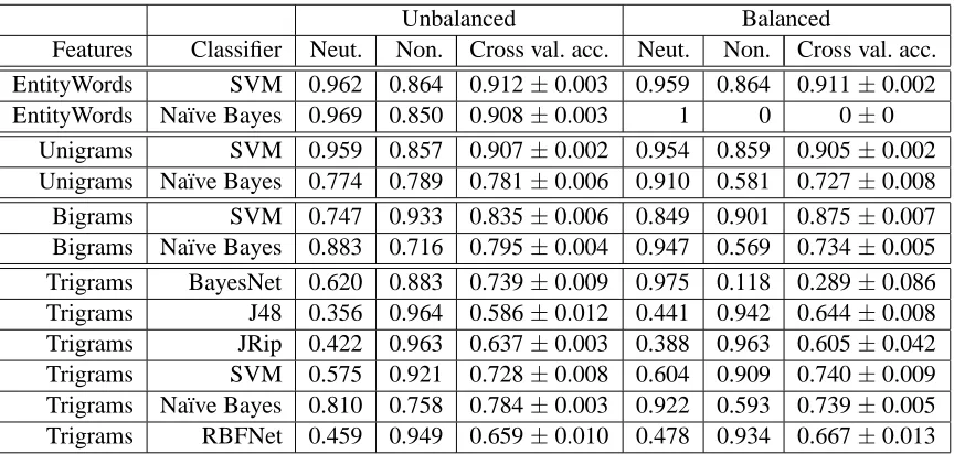
Finally, we look at our results considering the im-balanced data problem. Within some of the algo-rithms, balance is actively taken account during the training process: e.g. na¨ıve Bayes has a weighting on its class output to compensate for different fre-quencies, and the SVM training process uses geo-metric mean for computing performance, which en-courages a good performance on imbalanced data. In addition, we have presented results on the differ-ence between training with balanced and unbalanced datasets. Better results are obtained in 5 out of the 13 results for the pseudo-subjectivity task (Table 5), and in 6 out of 9 results for the pseudo-sentiment task (Table 6), suggesting that balancing the training data is a useful technique in most cases.
Unbalanced Balanced
Features Classifier Neut. Non. Cross val. acc. Neut. Non. Cross val. acc.
EntityWords SVM 0.962 0.864 0.912±0.003 0.959 0.864 0.911±0.002
EntityWords Na¨ıve Bayes 0.969 0.850 0.908±0.003 1 0 0±0
Unigrams SVM 0.959 0.857 0.907±0.002 0.954 0.859 0.905±0.002
Unigrams Na¨ıve Bayes 0.774 0.789 0.781±0.006 0.910 0.581 0.727±0.008
Bigrams SVM 0.747 0.933 0.835±0.006 0.849 0.901 0.875±0.007
Bigrams Na¨ıve Bayes 0.883 0.716 0.795±0.004 0.947 0.569 0.734±0.005 Trigrams BayesNet 0.620 0.883 0.739±0.009 0.975 0.118 0.289±0.086
Trigrams J48 0.356 0.964 0.586±0.012 0.441 0.942 0.644±0.008
Trigrams JRip 0.422 0.963 0.637±0.003 0.388 0.963 0.605±0.042
Trigrams SVM 0.575 0.921 0.728±0.008 0.604 0.909 0.740±0.009
Trigrams Na¨ıve Bayes 0.810 0.758 0.784±0.003 0.922 0.593 0.739±0.005
[image:8.612.91.523.70.276.2]Trigrams RBFNet 0.459 0.949 0.659±0.010 0.478 0.934 0.667±0.013
Table 7: Selected balanced versus unbalanced cross validation accuracies (geometric mean) for dataset S, pseudo-subjectivity task, together with the accuracies on the individual classes, neutral and non-neutral. For consistency, only results where attribute selection was performed are shown.
Unbalanced Balanced
Features Classifier Neut. Non. Cross val. acc. Neut. Non. Cross val. acc.
EntityWords SVM 0.872 0.394 0.587±0.006 0.575 0.812 0.683±0.007
EntityWords Na¨ıve Bayes 0.972 0.111 0.326±0.021 0.944 0.192 0.426±0.015
Unigrams SVM 0.837 0.464 0.622±0.011 0.694 0.698 0.696±0.005
Unigrams Na¨ıve Bayes 0.896 0.318 0.531±0.018 0.736 0.582 0.652±0.012
Bigrams SVM 0.852 0.36 0.553±0.006 0.58 0.8 0.68±0.012
Bigrams Na¨ıve Bayes 0.959 0.203 0.439±0.017 0.86 0.433 0.605±0.024
Trigrams SVM 0.935 0.173 0.401±0.018 0.407 0.851 0.588±0.009
Trigrams Na¨ıve Bayes 0.938 0.249 0.481±0.013 0.84 0.446 0.61±0.011
Table 8: Selected balanced versus unbalanced cross validation accuracies (geometric mean) for dataset A, pseudo-subjectivity task (see the preceding table for details).
A, and 88:12 for S).
Given these results, we suggest that balancing the training datasets is usually an effective strategy, al-though sometimes the benefits are small if account of balancing is also part of the parameter-selection process for your learning algorithm.
5 Conclusion and Further Work
We have empirically analysed a range of machine-learning techniques for developing favourability classifiers in a commercial context. These tech-niques include different classification algorithms, use of attribute selection to reduce the feature sets,
[image:8.612.91.522.330.482.2]References
A. Balahur, R. Steinberger, M. Kabadjov, V. Zavarella, E. Van Der Goot, M. Halkia, B. Pouliquen, and J. Belyaeva. 2010. Sentiment analysis in the news. In Proceedings of LREC.
A.L. Blum and P. Langley. 1997. Selection of relevant features and examples in machine learning. Artificial intelligence, 97:245–271.
N.V. Chawla, N. Japkowicz, and A. Kotcz. 2004. Edi-torial: special issue on learning from imbalanced data sets. ACM SIGKDD Explorations Newsletter, 6:1–6. G. Forman. 2003. An extensive empirical study of
fea-ture selection metrics for text classification. The Jour-nal of Machine Learning Research, 3:1289–1305. M. Gamon, A. Aue, S. Corston-Oliver, and E. Ringger.
2005. Pulse: Mining customer opinions from free text. Advances in Intelligent Data Analysis VI, pages 121– 132.
N. Godbole, M. Srinivasaiah, and S. Skiena. 2007. Large-scale sentiment analysis for news and blogs. In Proceedings of the International Conference on We-blogs and Social Media (ICWSM).
P.D. Green, P.C.R. Lane, A.W. Rainer, and S. Scholz. 2010. Selecting measures in origin analysis. In Pro-ceedings of AI-2010, The Thirtieth SGAI International Conference on Innovative Techniques and Applica-tions of Artificial Intelligence, pages 379–392. M. Koppel and J. Schler. 2006. The importance of
neu-tral examples for learning sentiment. Computational Intelligence, 22:100–109.
K. Krippendorff. 2004. Content analysis: An introduc-tion to its methodology. Sage Publicaintroduc-tions, Inc. M. Kubat, R.C. Holte, and S. Matwin. 1998. Machine
learning for the detection of oil spills in satellite radar images. Machine Learning, 30:195–215.
P.C.R. Lane, C. Lyon, and J.A. Malcolm. 2006. Demon-stration of the Ferret plagiarism detector. In Proceed-ings of the 2nd International Plagiarism Conference. T. Li, V. Sindhwani, C. Ding, and Y. Zhang. 2009.
Knowledge transformation for cross-domain senti-ment classification. In Proceedings of the 32nd in-ternational ACM SIGIR conference on Research and development in information retrieval, pages 716–717. ACM.
P. Melville, W. Gryc, and R. D. Lawrence. 2009. Sentiment analysis of blogs by combining lexical knowledge with text classification. In Proceedings of the 15th ACM SIGKDD international conference on Knowledge discovery and data mining, KDD ’09, pages 1275–1284, New York, NY, USA. ACM. D. Mladeni´c. 1998. Feature subset selection in
text-learning. Machine Learning: ECML-98, pages 95– 100.
T. Mullen and N. Collier. 2004. Sentiment analysis us-ing support vector machines with diverse information sources. In Proceedings of EMNLP, volume 4, pages 412–418.
B. Pang and L. Lee. 2008. Opinion mining and senti-ment analysis. Foundations and Trends in Information Retrieval, 2(1-2):1–135.
B. Pang, L. Lee, and S. Vaithyanathan. 2002. Thumbs up?: sentiment classification using machine learning techniques. In Proceedings of the ACL-02 conference on Empirical methods in natural language processing-Volume 10, pages 79–86. Association for Computa-tional Linguistics.
R. Prabowo and M. Thelwall. 2009. Sentiment analy-sis: A combined approach. Journal of Informetrics, 3:143–157.
M. Rogati and Y. Yang. 2002. High-performing feature selection for text classification. In Proceedings of the eleventh international conference on Information and knowledge management, pages 659–661. ACM. G. Tatzl and C. Waldhauser. 2010. Aggregating
opin-ions: Explorations into Graphs and Media Content Analysis. ACL 2010, page 93.
P.D. Turney. 2002. Thumbs up or thumbs down?: Se-mantic orientation applied to unsupervised classifica-tion of reviews. In Proceedings of the 40th Annual Meeting on Association for Computational Linguis-tics, pages 417–424. Association for Computational Linguistics.
X. Wan. 2009. Co-training for cross-lingual sentiment classification. In Proceedings of the Joint Conference of the 47th Annual Meeting of the ACL and the 4th International Joint Conference on Natural Language Processing of the AFNLP: Volume 1-Volume 1, pages 235–243. Association for Computational Linguistics. I. H. Witten and E. Frank. 2005. Data Mining: