Munich Personal RePEc Archive
Interpersonal Bundling
Chen, Yongmin and Zhang, Tianle
University of Colorado at Boulder, Lingnan University
23 May 2014
Interpersonal Bundling
Yongmin Cheny Tianle Zhangz
Revised March 5, 2014
Abstract. This paper studies a model of interpersonal bundling, in which a monopolist o¤ers a good for sale under a regular price and a group purchase discount if the number of consumers in a group—the bundle size—belongs to some menu of intervals. We …nd that this is often a pro…table selling strategy in response to demand uncertainty, and it can achieve the highest pro…t among all possible selling mechanisms. We explain how the pro…tability of interpersonal bundling with a minimum or maximum group size may depend on the nature of uncertainty and on parameters of the market environment, and discuss strategic issues related to the optimal design and implementation of these bundling schemes. Our analysis sheds light on popular marketing practices such as group purchase discounts, and o¤ers insights on potential new marketing innovation.
Keywords: Interpersonal bundling, bundling, group purchase, group discount, demand uncertainty
yUniversity of Colorado, Boulder, USA; [email protected] zLingnan University, Hong Kong; [email protected]
1. INTRODUCTION
This paper studies a form of product bundling where a good is o¤ered for sale under both a regular price and a group purchase discount if the group size—the bundle size— meets certain requirement. The de…ning characteristic of this selling format is that the purchase of the bundle is made by di¤erent consumers—and hence we term itinterpersonal bundling—rather than by a single consumer as under traditional mixed bundling.1
Interpersonal bundling (denoted as IB) is a widely observed selling practice. In many markets and for many goods, multiple consumers may form a purchase group to qualify for a group discount, as, for example, when buying tickets for a concert, purchasing a tour, or dining at a restaurant.2 In recent years, many Internet sites have emerged that allow sellers to o¤er IB, where consumers purchasing with group coupons receive substantial discounts when the minimum group size is reached. Launched in November 2008, Groupon was a pioneer in this selling format on the Internet, and it exceeded a billion dollars in revenue in just its third year of operation (Levin, 2012).3 Despite its popularity, the pricing and pro…tability of interpersonal bundling have not been studied in a general framework that allows a menu of bundle sizes. How should a seller optimally choose prices and bundle sizes? When will IB be more pro…table than separate selling?4 What determine the magnitude of
its pro…t advantage? We provide some answers to these questions in this study.
1Mixed bundling refers to o¤ering goods for sale both as a package and as individual components.
2Miller Farms, a local family farm in Colorado, runs the Fall Harvest Festival each year. In 2012, a
customer is charged $15 to participate in the Festival and pick up vegetables to take home. For a group of
10 or more, the price per person is lowered to $13.
3Many other group buying websites o¤er variants of interpersonal bundling, including Livingsocial, where
a consumer receives a free deal if she gets three people buy the product. There are numerous interpersonal
bundling sites around the global, such as uBuyiBuy, Gaopeng, and Lashou in Asia, MyCityDeal in Europe,
Downtown Colombia in South America, and Spreets in Australia.
4Here, separate selling means o¤ering a good for sale under a single unit price to all consumers, whereas
a pure bundle would consist of multiple units of the same good under a unit price for group purchase.
The recent economics literature has investigated product bundling that is di¤erent from traditional mixed
bundling. See, for example, the study of bundle size pricing by Chu, Leslie, and Sorensen (2011), and of
The literature on product bundling has found that mixed bundling often is more pro…table than separate selling through two main mechanisms: segmenting the consumer population to facilitate price discrimination and reducing the dispersion of consumer values to extract consumer surplus (e.g., Adams and Yellen 1976; Schmalensee, 1984; Long, 1984; McAfee, McMillan, and Whinston 1989; and Chen and Riordan, 2013).5 This paper will explore an
alternative motive for bundling: as a pro…table strategy in response to demand uncertainty. While this motive can also arise when each bundle is purchased by an individual consumer,6
it is especially relevant and important for interpersonal bundling.
We consider a stylized model where a monopolist sells to a population of low- and high-value consumers, with the numbers of these consumers being uncertain and following some joint probability distribution. Under separate selling, the seller wouldideallypursue a high-price strategy if high-value consumers is numerous, or a low-high-price strategy that will also attract low-value consumers if their number is su¢ciently large. However, because price is set before the uncertainty is resolved, a single price is generally not optimal. By o¤ering the good for sale under IB, it is possible that a high or low price will become e¤ective only when that price is optimal under the demand realization. Thus, interpersonal bundling potentially enables the seller to use optimal option pricing under uncertain demand, leading to higher pro…t than separate selling.
Our analysis of this model, in a general setting where the seller can commit to a menu that speci…es multiple bundle size intervals to which the group discount applies, leads to two results. First, we show that a bundle menu with at most two (disjoint) intervals is more pro…table than separate selling, provided that demand uncertainty is relevant for the choice of optimal prices under separate selling. Second, under a plausible su¢cient condition, IB
5In a standard model of two goods, some consumers may value one good highly but another very little,
while others may value two goods together relatively highly, and values for the bundle may be less dispersed
than values for individual goods. By charging the former (who purchase only a single unit) a higher price
and the latter a bundle discount, mixed bundling generally leads to higher pro…t than separate selling.
6Under standard mixed bundling with two goods, there can be uncertainties on each individual consumer’s
valuation for the two goods, and mixed bundling can thus be viewed as a form of option pricing, where a
achieves the highest pro…t among all possible selling mechanisms. Both results are obtained without assuming functional forms on the joint distribution of consumer numbers, and they provide a general and elegant characterization of the properties of interpersonal bundling.
To gain insights on when the general conditions on the pro…tability of IB are satis…ed and how to implement IB in various market environments, we further study two especially simple forms of IB: interpersonal bundling with a minimum or maximum group size, denoted respectively as IBmin or IBmax. For each of them, we derive a su¢cient condition for its superiority over separate selling. Interestingly, these two conditions, both invariant to the functional form of the consumer distributions, reveal contrasting patterns of demand uncertainty. Speci…cally, relative to separate selling, IBmin tends to be more pro…table when the number of low-value consumers is more dispersed, whereas IBmax tends to be more pro…table when the number ofhigh-value consumers is more dispersed. On the other hand, their pro…tability is also a¤ected by some other aspects of the market environment in similar ways. We illuminate the intuition behind these …ndings, relate them to observed marketing practices, and suggest that IBmax, as a potentially pro…table marketing innovation, can be implemented similarly as IBmin on the Internet and through intermediaries such as Groupon and Amazon.
We further explore how a seller may incorporate additional strategic considerations in the design of IBmin, by explicitly modeling the decision process of individual consumers in two variants of the main model. In the …rst variant, we allow the possibility that some consumers are initially uninformed about the existence of the seller’s product. Then, in order to qualify for the group discount, informed consumers may take (costly) actions to transmit product information to the uninformed, and the seller can exploit this incentive in setting the bundle size. IBmin can thus increase the seller’s pro…t by facilitating the dissemination of product information.7
7This informational role of group buying has also been identi…ed and explored in Jing and Xie (2011),
but their model focuses on exogenously …xed group size and known demand. By contrast, bundle size is a
key decision variable in our analysis of IBmin, and demand uncertainty is a central feature of our model
In the second variant, we consider the possibility that high-value consumers need to incur transaction costs to sign up for group purchase. The seller may then partially segment the consumer population, charging the regular price to high-value consumers with high sign-up costs while attracting low-value consumers with the bundle discount. To allow for a richer modeling of consumers’ decision process, we consider two forms of IBmin in a two-period setting: a simultaneous format where the seller does not inform period-2 consumers how many buyers signed up in period 1, and a sequential format where the seller does. Hu, Shi and Wu (2013) …nd in a parallel setting that the seller prefers the sequential mechanism, because it encourages consumer participation by removing their uncertainty in period 2, which leads to higher group formation rates. Interestingly, in our case the seller, who aims to maximize pro…t, may instead prefer the simultaneous format. This is because the simultaneous format does not remove uncertainty to the high-value consumers, which facilitates price discrimination by discouraging them from obtaining the bundle discount.
In addition to o¤ering a new perspective on product bundling, this paper is also closely related to the literature on pricing under demand uncertainty. In Dana (1999, 2001), for example, demand can be either high or low. He …nds that a monopolist optimally o¤ers two prices, with only a limited quantity o¤ered under a low price, which is set for the low demand state. A high price then allows the …rm to extract additional consumer surplus when demand turns out to be high, in which case the limited quantity available at the low price will sell out so that some high-priced units will be purchased. Anand and Aron (2003), in an early study of web-based group buying, also consider a model with either a high or a low demand regime, represented by two linear demand functions. They demonstrate that group buying may enable the seller to set price-quantity schedules that optimize revenue under each demand regime, and that the pro…tability of group buying relative to posted pricing depends on whether the two linear demand functions are parallel or intersecting.8 Our paper departs from this literature by adopting a di¤erent analytical approach, capturing the group
8Also related are Gale and Holmes (1992, 1993), who study how a monopolist may use advance purchase
discounts to allocate capacity more e¢ciently in the presence of demand uncertainty. See also Dana (1998)
buying problem in a general bundling framework. One clear advantage of this approach is that it enables us to analyze group-discount schemes with minimum or maximum group sizes in a uni…ed model and to uncover the interesting relations between them. Additionally, we are concerned with the uncertainty of a di¤erent nature: there are both high- and low-value consumers, and the uncertainty is over their respective numbers. We believe that this captures plausible market environments faced by many …rms, complementary to the settings studied in other papers in this literature. Furthermore, our analysis leads to interesting new results on the pro…tability and optimal design of interpersonal bundling. Our paper thus contributes to the literatures on product bundling, on pricing under demand uncertainty, and, more generally, on the economics and management of marketing.
In the rest of the paper, we establish the two general properties of interpersonal bundling in section 2, and analyze in more detail its two simple forms, IBmin and IBmax, in sec-tion 3. Secsec-tion 4 explores the optimal design of IBmin incorporating addisec-tional strategic considerations of information dissemination and price discrimination. Section 5 concludes.
2. DEMAND UNCERTAINTY AND INTERPERSONAL BUNDLING
2.1 The Model
A monopolist o¤ers a product for sale. There are two types of consumers, high-value and low-value, whose product valuations are respectively H and L; with H > L > 0: A consumer’s type is her private information, and each consumer desires to purchase at most one unit. The numbers of low- and high-value consumers (denoted as L-consumers and
H-consumers) are respectivelyxandy;which are realizations of random variablesX andY
that have joint distribution functionG(x; y)on support[ax; bx] [ay; by];where0 ax < bx and 0 ay by: The marginal distribution functions of X and Y are Fx(x) and Fy(y); respectively:Production cost is normalized to zero, and the …rm maximizes expected pro…t.
Let xand y be the expected number of L- and H-consumers, respectively. Then
x= Z bx
ax
xdFx(x) ; y=
Z by
ay
We allow the possibility that either y = y is a constant or x = x is a constant; in which case G(x; y) degenerates toFx(x) orFy(y):9
As a benchmark, consider the case of separate selling where the …rm posts a single unit price to all consumers. Then, pro…t is higher under p = H if Hy > L(x+y) and under
p=LifHy < L(x+y):It follows that the optimal price and the corresponding pro…t are, respectively:10
ps= 8 <
:
H if x H
L 1 y
L if x > HL 1 y
; s= 8 <
:
Hy if x H
L 1 y
L(x+y) if x > HL 1 y
: (2)
Therefore, if the expected number ofL-consumers (x) is small, the …rm will only sell to the
H-consumers at ps=H;otherwise, it will sell to all consumers at ps =L.
Under interpersonal bundling (IB), the …rm sets a stand-alone unit price p;a discounted unit price under group purchaseq p;and a condition that the group discount becomes ef-fective if and only if the number of consumers belongs to the setB f[mi; Mi] :i= 1; :::; ng for some integern; with0 mi Mi<1.11 An example of B with two intervals (n= 2) is B =f[0;1]; [2;3]g: IB may also contain a bundle with a single interval, B = [m; M];
which further nests two special cases: (1) IB with a minimum group size, or IBmin: (p; q; m);
where each consumer can separately purchase the good at price p;but consumers who sign up for group purchase can buy at the discounted price q if and only if there are at least m
consumers in the group: (2) IB with a maximum group size, or IBmax: (p; q; M); where consumers who sign up for group purchase can buy at the discounted priceq if and only if the group size does not exceed M:
Except for Subsection 4.2, we assume that there is no transaction cost to join group
9At least one ofX andY is not a constant. We also allow X orY to be discrete random variables, in
which caseax and bx or ay and by correspond respectively to the smallest and largest values that can be
realized.
1 0For ease of exposition, when pro…t is the same underp=H andp=L;we assume ps=H:
1 1When G(x; y) is not continuous, some inequalities in the bundle size conditionsmi Bi Mi may
be strict. More generally, IB can take the form of a general bundling menu f(pi; Bi)g; where consumers
in bundle sizeBi are charged with price pi: In our simple context, we use our equivalent formulation for
purchase, which implies that ifq < p, all consumers will attempt to purchase at q.
2.2 Pro…tability of Interpersonal Bundling
We …rst demonstrate that a simple form of IB, withp=H; q=L;and someB containing at most two intervals; is generally more pro…table than separate selling under demand uncertainty.
Given (p; q; B);all consumers will purchase at price q ifx+y 2B and q L; whereas when x+y 2 B only H-consumers will purchase at price p ifL < p H;where B is the complement of set B:The …rm’s problem is to maximize (expected) pro…t:
max
q L<p H;B (p; q; B) =q
Z Z
B
(x+y)dG(x; y) +p Z Z
B
ydG(x; y): (3)
Since (p; q; B) weakly increases inp and q for anyB; the optimalp andq that maximize
(p; q; B) are p = H and q = L: Hence the …rm’s maximum pro…t under IB and the optimalB are:
max
B (H; L; B) ; B = arg maxB (H; L; B): (4) Since (H; L; B) = L(x+y) if B = [ax+ay; bx+by] and (H; L; B) = Hy if B =
(bx+by;1);we have s:Thus, same as mixed bundling, IB will always be at least as pro…table as separate selling.
The seller’s problem can be written as maximizing
(H; L; B) = L Z Z
x+y2B
(x+y)dG(x; y) +H Z Z
x+y2B
ydG(x; y)
= Z Z
x+y2B
[L(x+y) Hy]dG(x; y) +Hy
= L(x+y) + Z Z
x+y2B
[Hy L(x+y)]dG(x; y):
Our result below will assume a regularity condition on uncertainty: there exist (small) intervals 1 and 2 on [ax+ay; bx+by];where i can be a single number if G(x; y) is not continuous, such that
Pr x+y > H
Ly x+y2 1 = 1; Pr x+y < H
That is, conditional onx+ybelonging to 1; x+y > HLy;and conditional onx+ybelonging to 2; x+y < HLy: This assumption rules out trivial cases wherex+y is always higher or lower than H
Ly for (almost) all possible realizations of (x; y);in which case under separate selling the optimal price will be independent of the realization of (x; y):As it will become clear later, condition (5) holds quite generally; in fact, if it is not satis…ed, then separate selling will always be an optimal selling scheme (see the argument immediately following (14) in the next subsection), and the resolution of demand uncertainty will not a¤ect the choice ofps.
Proposition 1 Under (5), interpersonal bundling (H; L; B0); with B0 containing at most
two intervals, is more pro…table than separate selling.
Proof. Since under separate selling s= maxfHy; L(x+y)g;we show that there is some
B0 such that (H; L; B0) > s whether s = Hy or s = L(x+y); and B0 contains at most two intervals.
Suppose that s=Hy: Then, let B0 = 1;we have,
H; L; B0 = Z Z
x+y2 1
[L(x+y) Hy]dG(x; y) +Hy > Hy:
(The …rst inequality above is due to revealed preference, and the second to the de…nition of 1;which is a single interval and could be a single number if it is a mass point.)
Next, suppose instead that s = L(x+y): Then, let B0 =
2; which contains two intervals, withB0= 2:We then have
H; L; B0 =L(x+y) + Z Z
x+y2B0
[Hy L(x+y)]dG(x; y)
= L(x+y) + Z Z
x+y2 2
[Hy L(x+y)]dG(x; y)> L(x+y):
theL-consumers are not served, and adding a discounted priceLthat becomes e¤ective only if the realized consumer group size corresponds to a region whereps=L;which is ensured by the construction of bundle B0, leads to a higher expected pro…t than separate selling
under ps = H: Similarly, when ps = L; pro…t can be increased by also o¤ering a higher regular priceH that becomes e¤ective only if the realized consumer group size corresponds to a region where pro…t is higher under ps = H: Thus, IB implements pro…table option pricing under demand uncertainty, boosting pro…t.
Notice that for IB to dominate separate selling with ps = H, the bundle size is only required to satisfyx+y2 1;i.e.,m x+y M for somem M;and for IB to dominate
ps=L, the bundle size is only required to satisfyx+y2
2;i.e.,x+y m orx+y M for somem M:Therefore a pro…table bundleB0 contains at most two intervals. However,
B0 may not be the optimal bundle. IB with a more generalB can potentially achieve higher pro…t. In fact, as we show next, IB with a general bundle menu B is an optimal selling scheme if a plausible su¢cient condition is satis…ed.
2.3 Interpersonal Bundling as an Optimal Selling Mechanism
This subsection demonstrates that IB(H; L; B );withB =f[mi; Mi] :i= 1; :::; ng;is an optimal selling mechanism under the following su¢cient condition (explained shortly):
(x; y) :x+y > H
Ly = ; (x; y) :x+y H
Ly = ; (6)
where
[ni=1f(x; y): mi x+y Mig:
We prove this by …rst characterizing the seller’s highest possible pro…t under its information constraint, using a general mechanism design approach. We then show that optimal IB achieves this (constrained) …rst best under (6).
who will receive a unit of the good with probability ( ) by paying p( );12 and truth
reporting is optimal for the consumer. Given that there is a continuum of consumers, ( )
and p( ) will depend on and on some aggregate measure(s) of consumers. For the …rst best, we assume that a mechanism may depend on the realized total demand from each of the two types of consumers,xandy:13 Then, a mechanism speci…esf ( ;x; y); p( ;x; y)g:
The seller chooses f ( ;x; y); p( ;x; y)g to maximize
= Z Z
[xp(L;x; y) (L;x; y) +yp(H;x; y) (H;x; y)]dG(x; y); (7)
subject to individual rationality constraints
(L p(L;x; y)) (L;x; y) 0; (8)
(H p(H;x; y)) (H;x; y) 0; (9)
and incentive compatibility constraints
(L p(L;x; y)) (L;x; y) (L p(H;x; y)) (H;x; y); (10)
(H p(H;x; y)) (H;x; y) (H p(L;x; y)) (L;x; y): (11)
From standard arguments,p(L;x; y) =L so that theL-type receives no information rents, and (10) holds with p(H;x; y) L: From (11), which holds in equality at the optimum, and withp(L;x; y) =L;we have
p(H;x; y) (H;x; y) =H (H;x; y) (H L) (L;x; y): (12)
Thus (9) and (12) are the two remaining constraints. Substituting (12) into (7), with
p(L;x; y) =L;we obtain
= Z Z
f[xL y(H L)] (L;x; y) +yH (H;x; y)gdG(x; y);
1 2We can also allow a transfer payment when the consumer does not receive the good, but it would be
optimal for the seller to set this payment to zero.
1 3In reality, the seller may only be able to commit to prices based on aggregate demandx+y;but not
on individual values ofxandy;becausexandymay not be separately veri…able whilex+ypotentially is.
Thus the …rst-best pro…t is only a benchmark. Remarkably, as we show next, IB can achieve this …rst best
which increases in (H;x; y):Since constraint (9) is not less likely satis…ed with an increase in ; it follows that (H;x; y) = 1 at the optimum. Then, (9) and (12) become H p(H;x; y) =H (H L) (L;x; y);and the seller chooses (L;x; y) to maximize
= Z Z
f(x+y)L (L;x; y) +yH[1 (L;x; y)]gdG(x; y); (13)
which can be written as
= Z Z
[(x+y)L yH] (L;x; y)dG(x; y) +Hy:
Therefore, letting (L;x; y) = 1 whenever x +y > HLy and (L;x; y) = 0 whenever
x+y HLy;the highest possible pro…t that the seller can achieve is
= Z Z
x+y>H Ly
[(x+y)L yH]dG(x; y) +Hy: (14)
There are two cases to consider in (14): (i) ifx+y < HLyfor (almost) all(x; y);or ifx+y >
H
Ly for (almost) all (x; y);we have =Hy orL(x+y) respectively, and hence separate selling as a special case of IB would achieve the …rst best. And (ii), (x; y) :x+y > HLy
has a positive measure and (5) holds. Then > Hy: In either case, under condition (6),
(H; L; B ) withB =f[mi; Mi] :i= 1; :::; ngwill achieve the …rst-best :
= Z Z
x+y2B
[(x+y)L yH]dG(x; y) +Hy: (15)
We summarize the above with the following:
Proposition 2 Under (6);interpersonal bundling(H; L; B )withB =f[mi; Mi] :i= 1; :::; ng
is an optimal selling scheme.
a general interpersonal bundling scheme, the idea is to divide this set into regions corre-sponding to intervals ofx+y:With bundle sizes designed to match these intervals, IB can achieve the …rst-best pro…t, as in (15), and it is therefore an optimal selling scheme.14
Propositions 1 and 2 are complementary to each other. Proposition 2 shows that IB is an optimal selling method under (6), but it may not dominate separate selling, which is a special case of IB, and the optimal bundle might be rather complicated. By contrast, Proposition 1 shows that a simple form of IB is more pro…table than separate selling, provided that the regularity condition is satis…ed, but it does not address the issue of whether IB is an optimal selling scheme. Together, they imply that IB dominates separate selling and achieves the highest possible pro…t when (5) and (6) are both satis…ed.
While Propositions 1 and 2 shed light on the properties of IB in general, it is not explicit how they relate to the parameter values of the model and to observed marketing practices. We next turn to simpler forms of IB that have been or can potentially be used relatively easily in practice, to gain insights on when the conditions for these results are satis…ed and how to design IB in di¤erent market environments.
3. IB WITH A MINIMUM OR MAXIMUM GROUP SIZE
In this section, we discuss two especially simple forms of interpersonal bundling, IBmin and IBmax. One motivation for the study of IBmin is that it is a widely observed selling practice, popularized especially on the Internet by Groupon. After studying IBmin, we also examine IBmax As it turns out, the pro…tability condition for IBmax is interestingly connected to that for IBmin.
1 4Condition (6) is needed, essentially because the …rst-best mechanism can depend separately on xand
y; while IB can only condition prices on x+y: With (6), information about x+y is su¢cient for the
implementation of the …rst best. Notice that if (x; y) :x+y >H
Ly is empty, (6) obviously holds with
i= 1andm1 =M1:In general, while (6) holds naturally in many situations (as we illustrate later), it need
3.1 Pro…t Advantages of IBmin
Notice that IBmin (p; q; m) is equivalent to ps = q if m a
x +ay; and to ps = p if
m > bx+by:Thus IBmin is always at least as pro…table as separate selling. To investigate when IBmin is more pro…table than separate selling and how large its pro…t advantage is, we note that, from (3) and (4), under IBmin the seller maximizes:
max
m (H; L; m) =L
Z Z
x+y m
(x+y)dG(x; y) +H Z Z
x+y<m
ydG(x; y): (16)
Let now be the highest pro…t under IBmin. Condition (A1) below provides a su¢cient condition for > s:
1 +ax ay
< H
L < 1 + bx
by
: (A1)
Proposition 3 IBmin (H; L; m) is more pro…table than separate selling if (A1) holds.
Proof. From (A1), Hby < L(bx+by):Thus there exists"1 12 bx+by HLby >0 such that bx+by "1 > HLby: Hence, ifx+y 2 1 = [bx+by "1; bx+by]; x+y > HLby HLy: It follows that
Pr x+y > H
Ly x+y2 1 = 1:
Also from (A1), Hay > L(ax+ay): Thus there exist "2 12 HLay (ax+ay) > 0 such thatax+ay+"2 < HLay:Hence, ifx+y2 2= [ax+ay; ax+ay+"2]; x+y <
H Lay
H Ly: It follows that
Pr x+y < H
Ly x+y2 2 = 1:
Therefore, condition (5) is satis…ed, and hence IBmin is more pro…table than separate selling from Proposition 1.
will indeed strictly increase pro…t. Condition (A1) is thus invariant to the functional form of the joint distribution of X and Y; depending only on the upper and lower limits of the support for the distribution:It holds if the H=Lratio is relatively large compared toax=ay but small compared to bx=by. IBmin allows the …rm to sell at the low price only if pro…t is higher under the low price—otherwise the high price will prevail—thereby assuring a higher pro…t than separate selling.15
In many situations where group coupons are issued by sellers such as restaurants and hair salons, H could be considered as the regular price at which the seller has less uncertainty about the number of consumers. Thus the di¤erence betweenayandby tends to be relatively small:On the other hand, there might be more uncertainty about the number of consumers who will purchase at the sale price L; so the di¤erence between ax and bx tends to be relatively large. In such situations, condition (A1) is likely satis…ed.16
To illustrate and to make explicit pro…t comparisons, consider the example below:
Example 1 Suppose that X and Y are independently and uniformly distributed on [0;3]
and [1;2];respectively:Then, x =y= 32; ps =H if H 2L; ps =L if H <2L; and (A1)
holds if H < 52L: Under IBmin,
(H; L; m) L Z 2
maxf1;m 3g
Z 3
maxfm y;0g
(x+y)1
3dxdy+H
Z minfm;2g
1
Z minfm y;3g
0
y1 3dxdy:
Setting @ (H; L; m)=@m= 0;we …nd the optimal minimum bundle size as
m = 8 > > > < > > > : H
2L H; with > s if H 43L 3
2HL; with >
s if 4
3L < H <2:6L
5; with = s if 2:6L H
:
For instance, if L = 1 and H = 2; then m = 3 and = 3:3333 > s = 3; so IBmin
increases (expected) pro…t by about 11%:
1 5IfH=Lis too small, it may be optimal always to sell atps=L;so the option to sell at alternative prices
has no value. Likewise, ifH=Lis too large, it could be optimal always to sell atps=H;which would then
achieve the same pro…t as interpersonal bundling.
1 6We may view IBmin as allowing the seller to experiment with a lower price that will prevail only when
the number of purchasing consumers reaches a minimum size, or only when it is more pro…table than the
Several observations can be made in Example 1. First, condition (A1) is su¢cient, but not necessary, for the pro…tability of IBmin. In Example 1, while (A1) holds forH <2:5L;
IBmin is also pro…table when H2[2:5L;2:6L):
Second, (A1) is fairly tight as a su¢cient condition. WhenH 2:6L;IBmin is no longer pro…table. In this case, 32H
L 3
2(2:6) = 3:9: However, for any m 2 [3:9;5);the expected pro…t underx+y m;in which case all sales will occur at the discounted priceL;is lower than the expected pro…t under separate selling. Therefore, it is optimal for the seller not to o¤er the bundle, which is equivalent to setting a su¢ciently large bundle size (m 5). Third, when IBmin is pro…table, m increases in H but decreases in L: A marginal increase in mreduces the probability that the sale will occur at the low price (with a large volume) and raises the probability that the sale will occur at the high price. Thus, m ;
which balances these two e¤ects, increases with the high price and decreases with the low price.
We now turn to the question of how the advantage of IBmin, relative to separate selling, may vary with the market environment. We …rst consider how the ratio H=L; or the di¤erence between the reservation prices of the high- and low-value consumers, a¤ects the relative pro…tability of bundling.
Corollary 1 Suppose that (A1) holds and Lis …xed. Then, s exhibits an inverted-U
shape with respect to changes in H;…rst increasing and then decreasing, reaching maximum
at H= 1 +xy L:
Proof. When H < 1 +xy L; s = maxm (H; L; m) L(x+y): From (16),
(H; L; m)increases inHfor all interiorm:Thus, if (A1) holds so that > s,max
m (H; L; m) is also increasing in H; and so is s: Similarly, when H 1 +xy L; s = maxmR Rx+y m[L(x+y) Hy]dG(x; y);which decreases inH.
When H=L is low (or high), the pro…t advantage of IBmin is low relative to separate selling, because selling at price L (or H) is often more pro…table than at price H (or L);
H=L is at some intermediate level, implying more profound pro…t advantage of IBmin.17
We next consider how the dispersion of X a¤ects the pro…ts under IBmin. Intuitively, whenX is more dispersed, demand is more uncertain and the advantage of IBmin is larger. The result below shows that this is indeed the case under some conditions, assuming thatX
and Y are independent with the (marginal) distribution ofY beingFy(y);and comparing pro…ts under two di¤erent distributions ofX:
Following Johnson and Myatt (2006), we say that distribution F^x(x) is more dispersed than Fx(x) ifF^x(x) is a rotation of Fx(x) such that x ?x^ ()F^x(x) 7Fx(x) for some rotation point x:^ Under F^x(x) and Fx(x); respectively, let xF^ and xF be the expected values of X; ^bx and bx the upper limits of F^x and Fx;and m^ and m the optimal bundle sizes, where ^bx bx and xF^ xF. Let the corresponding pro…ts be ^ and under bundling;and ^s and s under separate selling.
Corollary 2 Suppose (A1) holds andF^xis a rotation ofFxsuch that: (i)Hy L y+xF^ ;
(ii) x^ m by; and (iii)Rabyy[Lm Hy]
h ^
Fx(m y) Fx(m y)
i
dFy(y) 0:Then,
^ ^s> s;that is, the pro…t advantage of IBmin relative to separate selling is larger
if X is more dispersed.
Proof. See the appendix.
Although the result seems intuitive, the comparison of pro…ts under F^x(x) and Fx(x) turns out to be subtle. Condition (i) ensures that ps =H under separate selling for both
^
Fx(x)andFx(x):Under (ii),F^x(x)< Fx(x)forx m y;so that more dispersion under
^
Fx leads to higher probabilities for higher realizations of x; and under (iii) this similarly holds on average weighted by the density of Y: All three conditions can be easy to verify. For instance, in Example 1, whereFx(x) = x3;these conditions are satis…ed for any rotation
^
Fx(x) = x with >3 and H=L 2 [(3 + )=3; 2.6); where m = 32HL > 3 > by = 2; and
^ x= 0.
1 7We have also considered a variant of our model in which the reservation prices of the two types of
consumers are random variables instead of constant values, with similar insights on the pro…tability of
IBmin. The assumption that the reservation prices take constant valuesH andLallows us to illustrate our
3.2 Pro…tability of IBmax and the Nature of Uncertainty
We now study IBmax, (p; q; M); which also weakly dominates separate selling, since it is equivalent to ps = q if M > b
x +by and to ps = p if M ax +ay: We …rst establish the pro…tability of IBmax and its pro…t advantage relative to separate selling, in parallel to and in comparison with the analysis for IBmin. We then discuss limited-quantity discount (LQD), which is closely related to IBmax, and comment on how to implement IBmax.
From (3) and (4), under IBmax the seller maximizes:
max
M (H; L; M) =L
Z Z
x+y M
(x+y)dG(x; y) +H Z Z
x+y>M
ydG(x; y): (17)
Let now be the highest pro…t under IBmax. As another application of Proposition 1, Condition (A1’) below provides a su¢cient condition for > s:
1 +bx by
< H
L < 1 + ax
ay
: (A1’)
Proposition 4 IBmax is more pro…table than separate selling if (A1’) holds.
Proof. From (A1’),Hay < L(ax+ay):Thus there exists"1 12 ax+ay HLay >0such thatax+ay "1 > HLay:Hence, ifx+y2 1 = ax+ay; ax+ay+HL"1 ;theny ay+HL"1 and
x+y ax+ay >
H
Lay+"1 H
L y L
H"1 +"1= H Ly:
It follows that
Pr x+y > H
Ly x+y2 1 = 1:
Also from (A1’), Hby > L(bx+by):Thus there exists "2 12 HLby (bx+by) > 0 such thatbx+by+"2 < HLby:Hence, if x+y2 2= bx+by
L
H"2; bx+by ;theny by L H"2 and
x+y bx+by <
H
Lby "2 H
L y+ L
H"2 "2 = H
Ly:
It follows that
Pr x+y < H
Therefore, condition (5) is satis…ed, and hence IBmax dominates separate selling from Proposition 1.
Note that (A1’) is more likely to hold if ay is small relative toax and by is large relative tobx;that is, ifY is more dispersed thanX: When the number of high-value consumers(y) tends to be either much lower or much higher than the number of low-value consumers(x), the seller wishes to set a low price to sell to all consumers if y turns to be low, but a high price to sell only to the high-value consumers ify turns out to be high. By specifying that the low price becomes e¤ective only when the consumer group does not exceed a certain size, the seller can implement pro…table option pricing, charging a low price when demand is low and a high price when demand is high.
By contrast, the su¢cient condition for IBmin to dominate separate selling, (A1), is more likely to hold ifay is large relative to ax andby is small relative tobx;that is, ifX is more dispersed than Y: Thus IBmax and IBmin are pro…table selling schemes in response to demand uncertainties of a di¤erent nature. IBmin tends to be pro…table when the total number of consumers and their (average) valuation are likely negatively correlated: a higher number of consumers is likely associated with more low-value consumers; IBmax tends to be pro…table when the total number of consumers and their (average) valuation are likely positively correlated: a higher number of consumers is likely associated with more high-value consumers.18
Moreover, for …xed L; it is straightforward to show that the pro…t advantage of IBmax (relative to separate selling) is an inverted-U function of H; reaching maximum at H = 1 +xy L; similar to that of IBmin: It can also be veri…ed that this pro…t advantage is more pronounced if Fy is more dispersed, similar to the larger pro…t advantage of IBmin when Fx is more dispersed. Hence, there is a version of Corollary 1 and of Corollary 2 for IBmax, and we omit their formal statements to avoid repetition.
We next further show that IBmin or IBmax is in fact an optimal selling scheme, if there
1 8IB may not be pro…table if neither (A1) nor (A1’) is satis…ed. For example, if L = 1; H = 2; and
(X; Y) = (1;10) or (2;12) with equal probability, then ps = 2 and s = 22;which cannot be improved
exists eitherm orM with one of the following monotonic properties on the entire support of (x; y):
(C1) x+y m if and only ifx+y H Ly; or
(C2) x+y M if and only if x+y H Ly;
where the inequalities may be strict if m orM is a mass point, and m (orM ) is in the interior of[ax+bx; ay+by]if it is not a mass point.
Condition (C1) holds, for example, if y is a constant, in which case m = x +y for
x y HL 1 :Obviously, (C1) can also hold ify is not a constant. For example, suppose
L = 10; H = 12;and (X; Y) takes either (0, 50) or (100, 0) with equal probability. Then (C1) holds with strict inequality and m = 50:
Condition (C2) holds, for example, if x is a constant, in which case M = x+y for
y x= HL 1 : For an example where x is not a constant, suppose L = 10; H = 12;
and (X; Y) takes either (0,100) or (50, 0) with equal probability. Then (C2) holds with
M = 50:
Note that condition (5), under which IB dominates separate selling, and condition (6), under which IB is an optimal selling mechanism, are both satis…ed when either (C1) or (C2) holds. Therefore, from Propositions 1 and 2, we have:
Corollary 3 (1) Under (C1), IBmin dominates separate selling and also achieves the
…rst-best pro…t. (2) Under (C2), IBmax dominates separate selling and also achieves the …rst-…rst-best
pro…t.
In general, however, neither (C1) nor (C2) is necessarily satis…ed. For example, suppose
(X; Y) can take three possible pairs of values with equal probability: (2;0); (3;3); and
(10;4);with L= 1and H = 2:Then, on the support of (x; y): x+y HLy ifx+y 2or ifx+y 14; butx+y < H
While IBmin has been used in the sale of many goods, IBmax does not appear common. But a related format of IBmax, limited-quantity discount (LQD), has been used in many markets. LQD sets a low price for a limited quantity and raises the price for the additional quantity exceeding the limit. This is a popular selling strategy by airlines, hotels, stadiums, theaters, and even department stores, as discussed and analyzed in Dana (1999, 2001).19
Dana (2001; page 650) gives the following example:
Suppose that demand will be either high or low, each with probability 1/2. Low demand consists of 50 consumers with a reservation value of $10, and high demand consists of 100 consumers with a reservation value of $12. The seller must set its prices in advance. Within his context, the following is an optimal selling strategy under zero marginal cost: print 50 tickets at a price of $10 and 50 tickets at a price of $12. This yields an expected pro…t of $800, higher than $750, the highest expected pro…t under a uniform price.
With IBmax, however, the seller can do even better in this example. Reformulating the example with the notations of our model, we haveL= 10,H= 12and (X; Y)takes either (50,0) or (0,100) with equal probability. IBmax with regular price12;discounted price 10;
and maximum group size M = 50 leads to an expected pro…t of $850: The seller o¤ers IBmax (12;10;50) to all consumers for simultaneous sign up. If the demand state is low, at most 50 consumers will sign up for group purchase and will all receive the discount price $10. If the demand state turns out to be high, more than 50 consumers will sign up, in which case the price becomes 12, and all 100 consumers pay the higher price.
Intuitively, when the group size exceeds the maximum limitM, under LQD the low price is still e¤ective for units up to M: If many of those who would purchase M units at the low price, when x+y > M; are high-value consumers (in the above example all of them are), the seller can do better with IBmax by making the low price unavailable if the group size exceedsM. On the other hand, if those who would purchaseM units at the low price, whenx+y > M;are mostly low-value consumers, LQD can potentially be more pro…table.
1 9Denote the pro…t under LQD by ~ (p; q; M);whereM is the limited quantity to which the lower price
q applies. In our context, since ~ (H; L;0) = Hy and ~ (H; L; bx+by) = L(x+y); LQD is at least as
One possible reason why LQD has seen wide applications but IBmax has not is that it is more di¢cult for a seller to commit to IBmax and to communicate it to potential buyers. However, IBmax does not seem much more di¢cult to implement than IBmin. For instance, a seller could announce in advance a sale price L that is e¤ective only if the number of orders it receives does not exceed M for a certain time period; and if it exceeds M ; all of those who still wish to purchase the good will need to pay the regular price H:The announcement can be made through some intermediary such as Groupon or Amazon, and the number of orders received will be kept con…dential until the time period expires (so that consumers essentially submit orders simultaneously). The goods could be theater or sports tickets, vacation packages, restaurant meals, consumer electronics, and so on. Thus, we believe that IBmax, like many other marketing innovations, will potentially …nd its pro…table applications in the marketplace after it is conceived by researchers and understood by practitioners.
4. INFORMATION DISSEMINATION AND PRICE DISCRIMINATION
Our main model has focused on the role of demand uncertainty in the pro…tability of interpersonal bundling. Demand uncertainty is a common phenomenon in many markets, and our analysis demonstrates how …rms can use this selling strategy to increase pro…t in such market environments. In this section, we discuss how a seller may incorporate two additional strategic considerations in the design of IB to enhance its pro…tability, in two variants of the main model. We shall devote our attention to IBmin, due to its high relevance to the applications we have in mind, and also for the sake of keeping the discussions concise.
4.1 Dissemination of Product Information
To formalize this idea in a simple setting, we consider a variant of the main model by assuming that the number of H-consumers is initially a given number n 1; and each of them (i= 1; :::; n) can make an e¤ort in order to inform a set of k > 0 H-consumers who are initially unaware of the seller’s product and prices.20 De…ne set N fi:i= 1; :::; ng:
Each i2N succeeds in transmitting the information to the kuninformed consumers with probability i at a personal cost C( i);where C0( )>0 withC0(0)!0; C00( ) 0; and the k uninformed consumers become informed if at least one i 2 N succeeds. Thus, the number ofH-consumers is potentially
y= 8 <
:
n+k with probability 1 n
i=1(1 i)
n with probability n
i=1(1 i)
:
Other aspects of the model are the same as in Section 2. In particular, allL-consumers are informed about the seller’s product and price(s), and their number, x; is the realization of random variable X that has distribution F(x):(We drop the subscript x inF(x) for this section.) Under separate selling, informed consumers have no incentive to incur the cost to transmit product information. Hence ps = L and s = L(n+x) if L(n+x) > Hn; whereas ps=H and s=HnifL(n+x) Hn:
Under IBmin, the seller …rst posts(p; q; m);after which alli2N simultaneously choose
i:Both x and y are then realized, and possible purchases are made. For convenience, we again treat m as a continuous number, and without loss of generality, we can con…ne our search for the optimal (p; q; m) toq L < p H:
We consider a symmetric equilibrium where each i 2 N chooses the same : Given
(p; q; m); and all otherH-consumers’ choice ; i chooses her i to maximize her expected surplus:
U( ijm; ) = (H q)Pr(X+Y m) + (H p)Pr(X+Y < m) C( i);
2 0Unlike in Section 2, the number of initialH-consumers is now an integer. This avoids the problem that
no consumer is willing to incur the information transmission cost when the number is a continuum: For
where Pr(X+Y m) =
[1 F(m n k)]h1 (1 )n 1(1 i)
i
+ (1 F(m n)) (1 )n 1(1 i):
To see the trade-o¤ for i in choosing optimal i; notice that the optimal i satis…es
@U( ijm; )=@ ij
i= = 0 in a symmetric equilibrium, which, denoting the equilibrium
by (p; q; m) for any given(p; q; m), becomes:
(p q) [F(m n) F(m n k)] (1 )n 1 C0( ) = 0; (18)
where [F(m n) F(m n k)] is the increased probability of meeting m due to the addition of k uninformed consumers and (1 )n 1 is the probability that other (n 1) H-type informed consumers fail to reach the uninformed. Thus, as n goes to in…nitive, approaches zero because of the free riding problem. If nis …nite, however, rearranging the above equation gives
(p q) [F(m n) F(m n k)] = C
0( )
(1 )n 1:
Thus, for a …nite …xedn, the equilibrium = (p; q; m)is positive and increases in(p q)
becauseC00>0:The choice of balances the marginal bene…t of increasing the probability
of meeting the bundle size m and the marginal e¤ort cost of disseminating information. Holding other things constant, the bundle discount (p q) has to increase with n if the seller wishes to induce the same amount of e¤ort from the informed consumers. Hence, the …rm’s ability to use IBmin as an information dissemination device will be more limited when nbecomes larger.
Anticipating (p; q; m) in equilibrium, the seller will choose the equilibrium bundle
(p ; q ; m );and the equilibrium is then = (p ; q ; m ): In setting (p ; q ; m );the seller knows that IBmin now can increase pro…t for two distinct reasons. First, as a prof-itable pricing strategy under uncertainty, it increases pro…t even if i = 0for alli(in which case uninformed consumers do not learn about the product information). From Proposition 3 and (A1), this is ensured if
1 +ax n <
H
L < 1 + bx
Second, IBmin can motivate consumers to transmit product information to the unin-formed, or to choose i >0at a personal cost. In choosingm to provide this incentive, the seller balances two opposing e¤ects: while a highermmotivates the informed consumers to disseminate information, it may also diminish this incentive if the threshold is set too high. Our next result, which provides a su¢cient condition for higher pro…t under IBmin with the additional channel of encouraging information transmission to expand demand (i.e., in equilibrium i = >0), refers to the following condition:
1 +ax n <
H
L 1 + bx
n+k : (A2’)
Note that (A2’), which implies the weaker condition (A2), similarly holds if H=L is in an intermediate range.
Proposition 5 Suppose that (A2’) holds. Then, IBmin has higher pro…t than separate
selling with >0; p =H; and m 2(n+ax; n+k+bx):
Proof. See the appendix.
Since the discount price can be valid only if m is reached, the informed consumers have the incentive to transmit costly product information to the uninformed, hoping that more consumers will join the group purchase. As is shown in the proof for the symmetric equilibrium contained in the appendix, it is indeed optimal for each informed consumer to choose ; given that other informed consumers will do the same, and there exists an interior minimum size m . It is worth emphasizing that the optimalm is now chosen also to provide the incentive for , in addition to responding optimally to demand uncertainty. In other words, IBmin also provides a mechanism to expand market demand.
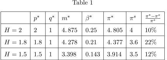
To illustrate, consider the next example:
Example 2 Suppose that n = 2; k = 1; C( i) = 12 2i; F(x) = x
3 for x 2 [0;3]; and
L < H < 52L: Then, condition (A2) is satis…ed, which is su¢cient for IBmin to increase
pro…t. With L = 1; Table 1 below lists the equilibrium bundle and the pro…t comparisons
Table 1
p q m s s
s
H = 2 2 1 4:875 0:25 4:805 4 10%
H = 1:8 1:8 1 4:278 0:21 4:377 3:6 22%
H = 1:5 1:5 1 3:398 0:143 3:914 3:5 12%
As in Example 1, given L; m is higher for higherH: Furthermore, is also higher for higherH;directly because of the larger bundle discount (H L), and indirectly because of the higher bundle size (m ):
For tractability, our model of information dissemination has made some simplifying as-sumptions. In particular, our assumption that each informed consumer can transmit sale information to all uninformed consumers with some probability is restrictive. While it is possible that an informed consumer can publicize the group coupon information to all un-informed consumers through media such as facebook or an online forum, our assumption is made mainly for the tractability of analysis. We expect that the basic insights will still be valid in a more realistic setting where various numbers of uninformed consumers may become informed with di¤erent probabilities.
Another of our simplifying assumptions is that the uninformed are allH-consumers. One may wonder what would happen if some L-consumers were also in the uninformed pool. To see this most strikingly, suppose that the uninformed are all L-consumers. Then, the incentive for the informed H-consumers to disseminate information remains unchanged, because both types of consumers are willing to buy at the discounted priceL. However, the …rm’s problem would need a slight modi…cation: ifm is reached, the …rm would earn pro…t
to disseminate information.21
4.2 Price Discrimination
To obtain the group discount under IB, a consumer may need to incur transaction costs to sign up for group purchase. If H-consumers have higher time costs, they are less likely to participate. Interpersonal bundling can thus be a device for price discrimination, as in the textbook example of price discrimination through coupons. With IBmin, however, there is an additional instrument to screen the buyers: Through the choice of the minimum bundle size that may not be reached due to uncertainty, the seller can further discourage
H-consumers from attempting to receive the group discount.
To illustrate, consider another variant of the main model, where the L-consumers have no cost to participate in group purchase, but theH-consumers incur a transaction costtto do so. Assume thattis distributed on[t; t]with p.d.f. (t)>0;c.d.f. (t);and 0 t < t:
The number of L-consumers is again x with cumulative distribution function F(x); while the mass of H-consumers is normalized to 1. Under separate selling, ps = H = s if
H L(x+ 1);whereas ps=L and s=L(x+ 1) ifH < L(x+ 1):
As in the main model, the game under IBmin proceeds as follows: First, the seller o¤ers
(p; q; m): Second, the number of L-consumers and the private t for each H-consumer are realized. Third, consumers choose whether to sign up for group purchase. Fourth, the total number of consumers who sign up becomes known. If this number exceeds m; each group member paysqwhile consumers who have not signed up will payp;otherwise, all consumers are charged regular pricep.
In order to analyze price discrimination under alternative forms of IBmin, we further assume that consumers can sign up for group purchase possibly in two periods, 1, or 2. (Neither the seller nor consumers discount time.) Under the simultaneous format, at the beginning of period 2 the seller does not reveal how many consumers signed up in the …rst
2 1The analysis can also be properly modi…ed to deal with the more general case where the uniformed were
a mix of the two types of consumers, and 2[0;1]were the portion of theH-consumers in the uninformed
period, whereas under the sequential format the …rm does. Hence, with the former all consumers e¤ectively make sign-up decisions simultaneously, whereas with the latter they make sign-up decisions sequentially.
Simultaneous Format
In this case, anH-consumer, if she wishes to participate, needs to incurtbefore it becomes known how many L-consumers have joined group purchase, or what the realization of x is (it is optimal for all L-consumers to sign up for group coupon since they incur no sign-up cost). Suppose that there is somet 2[0; t]that solves
H p= Z
x+ (t ) m
(H q)f(x)dx+ Z
x+ (t )<m
(H p)f(x)dx t : (19)
Then, there will be an equilibrium where allL-consumers sign up for group purchase, and an H-consumer will sign up if and only if t t :22 We shall focus on this equilibrium.23 Rearranging (19), we obtain
t = (p q) [1 F(m (t ))]: (20)
The seller’s problem is, witht =t (p; q; m);to maximize
(p; q; m) = Z bx
m (t )
[q(x+ (t )) +p(1 (t ))]f(x)dx+p
Z m (t )
ax
f(x)dx (21)
subject to q L; L p H; ax m (t ) bx: The solution to (21) de…nes the equilibrium (p ; q ; m ):
With regular price p and discounted bundle price q, an H-consumer may nevertheless prefer to purchase atp;because she incurstfor group purchase and she may losetwithout receiving the bundle discount if m is not reached. Hence, a higher m will reduce the incentive of anH-consumer to engage in group purchase. IBmin may thus price discriminate more e¤ectively both than traditional coupons and than traditional mixed bundling. A
2 2Equation (19) says that the marginalH-consumer witht will just be willing to sign up;given(p; q; m)
and given the equilibrium behavior of all other consumers.
2 3There can also be a trivial equilibrium where no one signs up for the group coupon, due to there being
higher m; however, can hurt the seller if the sales to the L-consumers do not materialize. Notice that any q belowL will lower the seller’s pro…t when the good is sold at a discount and will also make participating in group purchase more attractive to the H-consumers. Thus it is optimal for q =L:On the other hand, a higher p may increase the pro…t from the H-consumers paying p but makes the bundle discount more attractive. Consequently, the optimalp is determined jointly withm:
Again denote the seller’s equilibrium pro…t under IBmin by : To derive a su¢cient condition under which > s;we utilize the condition below
(i) t > H L; (ii) H
L <1 + bx
(H L): (A3)
Since p H; part (i) in (A3) ensures that some H-consumers will not incur t for the bundle discount, and, from (21),
(H; L; ax) =L[x+ (H L)] +H[1 (H L)]> L(x+ 1) = sjps=L;
so that (p; q; m) = (H; L; ax) is always more pro…table thanps =L: Moreover, since t
H L and part (ii) in (A3) implies H (t ) < L[ (t ) +bx], if m = bx+ (t ) " for small enough" >0(i.e., mis slightly belowbx+ (t ), we have, from (21):
(H; L; bx+ (t ) ") =
Z bx
bx "
[L(x+ (t )) H (t )]f(x)dx+H
Z bx
bx "
[L(bx "+ (t )) H (t )]f(x)dx+H > H = sjps=H;
where the last inequality above holds because H (t ) < L[bx+ (t ) "]for su¢ciently small ": Hence (p; q; m) = (H; L; bx+ (t ) ") is always more pro…table than ps = H: Therefore, since ps = L or H; under condition (A3) it must be true that > s and
p > L=q . We have thus established:
Proposition 6 Suppose that condition (A3) is satis…ed. Then, the seller’s pro…t is higher
under IBmin than under separate selling with p > L=q .
Notice that sinceyis normalized to 1 in this variant of the model, (A1) becomes(1 +ax)<
t > H L:IBmin dominates separate selling under broader conditions here than in the main model, because it now may increase pro…t also through price discrimination. To illustrate, supposeH=L <1 +ax:In this case, if, as in the main model, no consumer has sign-up costs, IBmin is not pro…table and the …rm will optimally choose ps =L. However, with positive sign-up costs for H-consumers, IBmin becomes pro…table through price discrimination. In fact, bundle (H; L; ax); under which m = ax is always reached but H-consumers with
t > H L will choose not to join the group and will hence pay price H; yields a higher pro…t than separate selling. (The seller may do even better by optimally choosing somem
that is di¤erent fromax.)
Sequential Format
Now consider the sequential format: Since an L-consumer has no cost to sign up, it is optimal for her to do so in the …rst period. Therefore in equilibrium allL-consumers sign up in period 1 and their number is then publicly known.
Next consider the sign-up decision of H-consumers, for whom it is optimal to wait until the beginning of period 2 to make the choice.24 Suppose for a moment that, in equilibrium,
depending on the realization of x, there exists a cuto¤ value t (x) such that only H -consumers with t t will sign up for group purchase. Given such a strategy by other consumers, an H-consumer with sign-up cost t chooses to sign up only if this leads to a (weakly) higher surplus for her and if a group discount is expected to be o¤ered:
H q t H p and x+ (t ) m:
Hence the marginal H-consumer has t=p q. It follows that, if x x^, it is optimal for any H-consumer witht t to sign up given that the others will do the same, where
t =p q and x^=m (p q); (22)
2 4In reality, it might also be costly for anH-consumer to learn how many consumers have already joined
the group, possibly because of the cost to visit the sign-up website. For convenience, we assume that t
is incurred when the consumer actually signs up for group purchase, such as transaction costs to open an
and the group size will be reached. Therefore, under the sequential format, there is indeed an equilibrium, where the seller chooses (p; q; m) optimally, L-consumers sign up in the …rst period, and: (i) if x x;^ then H-consumers with t t will sign up in the second period and m will be reached, so that group participants will pay discounted priceq while non-participants (H-consumers with t > t ) will pay regular price p; (ii) if x < x;^ no
H-consumers will sign up and only regular pricep is available.25
Comparing (22) with (20), we have t > t : That is, more H-consumers will sign up for group purchase under the sequential than under the simultaneous format of IBmin. This implies that, for the same bundle, group purchases will occur more often under the sequential format. The intuition behind this …nding, as in Hu, Shi, and Wu (2013), is that the sequential format removes the uncertainty faced by period-2 consumers about the number of participating consumers in period 1, which makes period-2 consumers more willing to sign up. Although our model and analysis di¤er from those in Hu, Shi, and Wu (2013),26
our …nding supports their conclusion that the sequential group-buying mechanism will lead to higher deal success rates. While this implies that a seller would prefer the sequential format if, as they assume, it aims to maximize the deal success rates, in our model the seller, whose objective is to maximize pro…t, may actually prefer the simultaneous format. To see that pro…t can be higher under simultaneous than under sequential IBmin, we notice that the seller’s pro…t function for the sequential format can be obtained by using the pro…t expression for the simultaneous format in (21) but replacing t witht :
(p; q; m) = Z bx
m (t )
[q(x+ (t )) +p(1 (t ))]f(x)dx+p
Z m (t )
ax
f(x)dx:
(23) While a complete comparison of pro…ts under the two formats is rather complicated and
2 5Potentially there can also be an equilibrium in which some of theH-consumers with lowtsign up in the
…rst period, which may enhance the probability of a discrete bene…t of the group discount. In the appendix,
we argue that this equilibrium, when it exists, has qualitatively similar properties as the equilibrium here.
2 6Among other di¤erences, in their group-buying mechanisms consumers have heterogenous valuations
but identical participation costs, whereas in our model high-value consumers di¤er in participation costs but
beyond the scope of our paper, we demonstrate that pro…t can be higher in the simultaneous format with the following example:
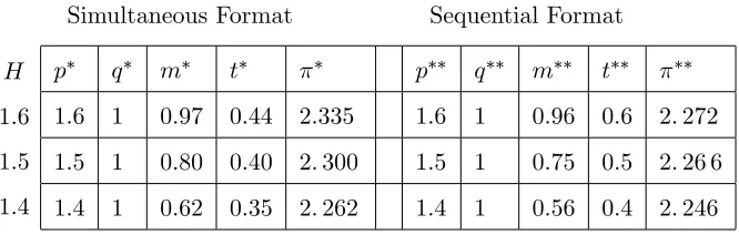
Example 3 Assume that (t) = 1 on [0;1]; f(x) = 21 on [0;2]; and L= 1: For di¤erent
values ofH;Table 2 compares equilibrium simultaneous and sequential IBmin, denoted with
[image:33.612.153.486.258.364.2]superscripts and ;respectively.
Table 2
Simultaneous Format Sequential Format
H
1:6
1:5
1:4
p q m t p q m t
1:6 1 0:97 0:44 2:335 1:6 1 0:96 0:6 2:272
1:5 1 0:80 0:40 2:300 1:5 1 0:75 0:5 2:26 6
1:4 1 0:62 0:35 2:262 1:4 1 0:56 0:4 2:246
Example 3 makes it clear that a pro…t-maximizing seller may prefer the simultaneous over the sequential format. This is because the seller wishes to price discriminate when using IBmin, and, unlike the sequential format, the simultaneous format does not remove uncertainty for theH-consumers, thereby discouraging them from signing up to obtain the group discount.
5. CONCLUDING REMARKS
high-value) consumers is more dispersed. Furthermore, the pro…tability of IBmin will be enhanced if the incentive to qualify for group purchase motivates buyers to disseminate product information, and if more high-value consumers can be induced to pay the regular instead of the discounted price.
Like other selling formats, interpersonal bundling can achieve its potential bene…ts for the seller only if it is properly implemented. In particular, losses may occur if the bundle discount under group purchase is too big. For example, when a restaurant o¤ers a group coupon for 70% o¤ its regular price, it could be unwisely pricing below marginal cost.27 While many businesses have pro…ted from o¤ering IBmin on the Internet, there have also been media reports about how a merchant is hurt by its deep group discount through Groupon and other “social buying” intermediaries.28 Part of the problem is a potential
con‡ict in incentives: even though the seller should use the advertised deal to maximize its pro…t, an intermediary like Groupon bene…ts from a higher deal success rate. However, it need not be in the best interests of the sellers (and, in the long run, also their Internet intermediaries such as Groupon) to focus only on deal success rates. As our theory suggests, the seller’s pro…t is sometimes higher when the deal is o¤—–if the realized number of low-value consumers is not high.29 And, it would be even worse for sellers if below-cost group
sale prices are used to boost deal success rates.
We have studied monopoly interpersonal bundling in this paper. It would be desirable
2 7The restaurant may want to attract repeat customers by taking a one-time loss, but is the loss necessary?
Our analysis suggests that interpersonal bundling can be pro…table without the repeat-business e¤ect, and
a seller need not incur losses in order to generate repeat businesses.
2 8See, for example, “Groupon demand almost …nishes cupcake-maker” (November 22, 2011, The
Tele-graph), which tells the story of a British cakemaker who o¤ered her product at 75% o¤ its regular price
through Groupon and had to produce at costs substantially above price in order to meet a huge demand
increase. See also Byers, Mitzenmacher and Zervas (2012) for discussions about negative side e¤ects for
merchants using Groupon.
2 9As a form of advertising, IBmin on the Internet can also serve as a promotional device that encourages
consumers to try the product and become repeat customers. While we do not model such roles, they can
also be important. Indeed, some sellers may have used Groupon as an advertising platform to attract repeat
APPENDIX
Proof of Corollary 2. From (i), Hy L y+xF^ : Hence under separate selling the optimal price isH for eitherF^x orFx:It follows that
^ ^s = Z Z
x+y m^
[L(x+y) Hy]dF^x(x)dFy(y) +Hy Hy
Z by
ay
(Z ^bx
m y
[Lx (H L)y]dF^x(x)
)
dFy(y);
where the inequality is due to revealed preference. Since F^x(x) < Fx(x) for x m y from (ii), we have
Z ^bx
m y
[Lx (H L)y]dF^x(x)
= hL^bx (H L)y
i
[Lm Hy] ^Fx(m y)
Z bx
m y
LF^x(x)dx
Z ^bx
bx
LF^x(x)dx
> [Lbx (H L)y] [Lm Hy] ^Fx(m y)
Z bx
m y
LFx(x)dx:
Thus
^ ^s > Z by
ay
[Lbx (H L)y]dFy(y)
Z by
ay
[Lm Hy] ~Fx(m y)dFy(y)
Z by
ay
Z bx
m y
LFx(x)dxdFy(y):
(from (iii))
Z by
ay
[Lbx (H L)y]dFy(y)
Z by
ay
[Lm Hy]Fx(m y)dFy(y)
Z by
ay
Z bx
m y
LFx(x)dxdFy(y)
= Z bx
m y
Proof of Proposition 5. First, in equilibrium, i satis…es (18). The …rm’s problem is:
max
q L<p H;m (p; q; m) (24)
= q [1 (1 )n] Z
x m n k
(x+n+k)dF(x) + (1 )n Z
x m n
(x+n)dF(x)
+p[[1 (1 )n] (n+k)F(m n k) + (1 )nnF(m n)]:
Next, from (18) and with C00 0;we have (p; q; m) increasing in pand decreasing inq;and furthermore
@ (p; q; m)
@m =
(p q) [f(m n) f(m n k)] (1 )n 1
(n 1) (p q) [F(m n) F(m n k)] (1 )n 2+C00:
Thus (p; q; m) is increasing in m at m=n+ax but decreasing in m atm =n+k+bx: At the optimum, (p; q; m) must increase in :Thus, since (p; q; m) and (p; q; m) both increase inp;the solution to problem (24) must havep=H;so that problem (24) becomes
maxq L;m (H; q; m):Next,
@ (H; q; m)
@ = qn(1 )
n 1 Z
x m n k
(x+n+k)dF(x) Z
x m n
(x+n)dF(x)
+Hn(1 )n 1[(n+k)F(m n k) nF (m n)];
with
@
@ m=n+a
x
=qn(1 )n 1k >0; @
@ m=n+k+b
x
=Hn(1 )n 1k >0:
Next, since Hn L(n+ax) by assumption (A2’),
@ (H; q; m)
@m m=n+a
x
= [1 (1 )n] [H(n+k) qm]f(m n k)jm=n+ax
+ (1 )n(Hn qm)f(m n)jm=n+ax+ @ (p; q; m) @
@ (p; q; m)
@m m=n+a
x
@ (p; q; m)
@ m=n+a
x
@ (p; q; m)
@ m=n+k+b
x
>0:
On the other hand;atm=n+k+bx;@ (p;q;m@ )@ (@mp;q;m) <0; f(m n) = 0; f(m n k)>