Parameter estimation under uncertainty with Simulated Annealing applied to an ant colony based probabilistic WSD algorithm

Parameter estimation under uncertainty with Simulated

Annealing applied to an ant colony based probabilistic WSD

algorithm

Andon T CH ECH M EDJ I EV

_{Didier SCHWAB}

_J

_´

_er

ˆ

ome GOU LIAN

Gilles S

ERASSET

´

(1) Univ. Grenoble-Alpes, LIG-GETALP, France

{andon.tchechmedjiev, didier.schwab, jerome.goulian, gilles.serasset}@imag.fr

A

In this article we propose a method based on simulated annealing for the parameter estimation of probabilistic algorithms, where the solution provided by the algorithm can vary from execution to execution. Such algorithms are often very interesting to solve complex combinatorial problems, yet they involve many parameters that can be difficult to estimate manually due to their randomized output. We applied and evaluated a method for the parameter estimation of such algorithms and applied it for an Ant Colony Algorithm for WSD. For the evaluation, we used the Semeval 2007 Task 7 corpus. We split the corpus and took in turn one text as a training corpus and the four remaining texts as a test corpus. We tuned the parameters with an increasing number of sentences from the training text in order to estimate the quantity of data necessary to obtain an efficient and general set of parameters. We found that the results greatly depend on the nature of the text, even a very small amount of training sentences can lead to good results if the text has the right properties.

R

Estimation de paramètres à base de Recuit Simulé sous incertitude appliquée à un algo-rithmes à colonies de fourmis probabiliste.

Nous proposons une méthode basée sur un Recuit Simulé pour l’estimation de paramètres pour des algorithmes probabilistes où les solutions générées varient. Ces algorithmes sont souvent très intéressant pour la résolution de problèmes combinatoires complexes, mais ils requièrent de nombreux paramètres pouvant être difficiles à estimer manuellement à cause de la nature aléatoire des solutions. Nous avons appliquésPlus spécifiquement, nous appliquons et évaluons cette méthode à pour estimer les paramètres de tels algorimes et l’appliquons à un Algorithme à Colonies de Fourmis pour la désambiguïsation lexicale. Pour l’évaluation, nous avons utilisé le corpus de Semeval 2007 Tâche 7. Nous avons repectivement séparé un texte comme corpus d’entraînement et les quatre autres comme corpus de test. Nous estimons les paramètres pour un nombre croissant de phrases pour déterminer combien de données sont nécessaires pour obtenir un ensemble de valeurs de paramètres générales et efficaces. Nous concluons que la qualité des résultats dépends de la nature des textes. Même des petites quantités de de phrases peuvent suffir à obtenir de bons résultats, du moment que le texte à les bonnes propriètés. KEYWORDS:Word Sense Disambiguation, Parameter Estimation, Simulated Annealing, Uncertainty, Stochastic Algorithms.

KEYWORDS INFR: Désabiguïsation Lexicale, Estimation de Paramètres, Recuit Simulé, Incertitude,

1 Introduction

Word Sense Disambiguation (WSD) is a very difficult yet central task in Natural Language Processing (NLP), that pertains to the labelling of the words of a text with the senses that most closely match the context. Numerous approaches exist to tackle WSD, yet many of these methods have in common a sizeable complexity, reflected by a number of parameters that need to be tuned in order to obtain the best performance. Depending on the number of parameters, it can be very difficult for a human to directly estimate the optimal parameters. Even then, it remains a question of guesswork with no guarantee of success.

This issue is all the more salient with algorithms and models that typically involve many parameters upon which the results greatly depend. Such algorithms for WSD include Neural Networks (Veronis and Ide, 1990), Simulated Annealing (SA) (Cowie et al., 1992), Genetic Algorithms (GA) (Gelbukh et al., 2003) and Ant Colony Algorithms (ACA) (Schwab and Guillaume, 2011), and many other machine learning methods.

In such approaches, the values of the parameters are paramount. They are what make the algorithms work for specific applications such as WSD. Yet, the authors of the aforementioned articles give little insight as to how the parameters are determined. They only provide the “best” values. Although atrial and errorapproach is a good start when devising an algorithm or tailoring it to a new application, it makes the adaptation and the scalability of such systems an issue. Naturally, for well known and understood algorithms such as Simulated Annealing, there are some theoretical criteria to select the parameters. However, the process remains to be repeated for every new setting and can be tedious to perform.

Furthermore, even with few parameters, evaluating all possible parameter configurations is a prohibitively long process. For example, in the case of a stochastic algorithm with 10 parameters that have 20 possible values each, assuming the algorithm needs to be run 100 times (due to its stochastic nature) and that one execution takes on average 30 seconds, the time necessary to evaluate all parameter combinations is 2012

·100_×30=3_×1015_{swhich is almost 1 billion years! Thus, the advantages of considering automated} or adaptive heuristic approaches to the estimation of parameters are clear.

In the case of a deterministic algorithm, many combinatorial optimisation methods can be used with little effort. However, due to the complexity of WSD, many approaches are statistical or probabilistic in nature and the use classical combinatorial optimization heuristics becomes impossible. Therefore, we adapt the classical simulated annealing algorithm to work for an uncertain objective function based on the ideas of (Painton and Diwekar, 1995), by using standard non-parametric statistical significance tests.

First, we present the tools and the metrics for the evaluation of WSD, followed by the description of the Ant Colony Algorithm considered in this article. Then, we briefly survey other approaches for parameter estimation under uncertainty and express the problem formally. Subsequently, we present the general formulation or simulated annealing and different aspects pertaining to it and then present its adaptation to uncertain objective function. We then present and analyse our experimental protocol and the results of the experiments. Finally, we conclude on the results and draw some perspectives for future research.

2 Evaluation of WSD Systems

The use of Precision and Recall constitutes the standard evaluation metrics for WSD systems. Precision represents the number of correctly disambiguated words among all the attempted words, while Recall represents the number of correctly disambiguated words among all the ambiguous words in the document. It is customary to compute the F1 score between Precision and Recall as2·P·R

P+R, in order to have

keys. An algorithm must correctly tag as many ambiguous words as possible (T P) depending on the context. A sense is considered correct if the sense key assigned to it matches the sense provided in the gold standard or any of its subsumed senses (hence coarse-grained). If we write the number of incorrectly assigned senses as (T N), then, for this particular task, precision can be expressed asP=T PT P+T Nand recall

asR=T PT

The choice of the all words task in particular is based on the functioning of the algorithm that is more adapted to a globally coherent text, rather than independent sentences or words. As such, the metrics available for the evaluation are Precision, Recall and F-measure, which leads to some important restrictions on the methods or criteria available for parameter estimation as will be detailed in the subsequent sections.

3 Context: an ant colony algorithm for WSD

The ant colony algorithm presented by (Schwab and Guillaume, 2011) and (Schwab et al., 2012) that our work focuses on, offers some interesting properties regarding the quality of the solutions, which are on par with state-of-the-art knowledge rich WSD systems, combined with a fast execution time compared to the latter systems. Furthermore, it is also well suited to working on full texts at a time with a full annotation coverage.

Moreover, its stochastic nature leads to the generation of solutions with variable precision scores, which is usually not a very sought after property in algorithms. However, this variability enables the use of voting strategies that lead to results approaching supervised WSD systems and overcome the elusive (for unsupervised and knowledge-based systems) First Sense Baseline. Due to the quick execution time (in the 60s to 65s range), voting strategies can directly be applied while still leading to cumulative execution times for several executions that are lower to that of other systems.

However, those qualities are also a major disadvantage when it comes to selecting and tuning the parameters of the algorithm. Not only are there relatively many, but they can only be determined manually to some extent through painstaking trial and error modifications, with no guarantees of optimality. Notwithstanding with the fact that the stochastic nature of the algorithm makes it rather impractical to determine whether the improvement resulting from a given parameter change is simply due to random variations of the solution distribution or really to significant variations.

3.1 Parameter model

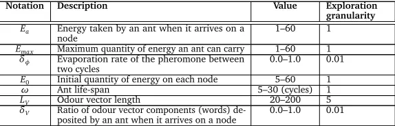
Let us now review the various parameters of the system, their typical value ranges and meaningful increments. The parameters are summarized in Table 2. There are seven parameters in total, five of which are discrete and represented by integers and two continuous parameters represented as positive real numbers between zero and one.

Given the number of parameters, even with some knowledge about how the algorithm works, one can at best chose sensible parameter value ranges in order to limit the combinatorial explosion.

Initially, before the estimation method proposed in this paper, we determined the values of some parameters by making iterative and independent changes. Of course such an approach is limited due to the fact that it is a heuristic based on the assumption that the parameters of the system are independent. For ACA it is in fact the opposite, as it is with other methods.

The values obtained through this process were ω=10,Ea=1,Emax =8,E0=10,δv=0.9,δ=

0.9,LV=90 and yielded results around 75% on the Semeval 2007 Task 7 corpus (Schwab and Guillaume, 2011).

Notation Description Value Exploration granularity

Ea Energy taken by an ant when it arrives on a

node 1–60 1

Emax Maximum quantity of energy an ant can carry 1–60 1

δφ Evaporation rate of the pheromone between

two cycles 0.0–1.0 0.01

E0 Initial quantity of energy on each node 5–60 1

ω Ant life-span 5–30 (cycles) 1

LV Odour vector length 20–200 5

δV Ratio of odour vector components (words)

de-posited by an ant when it arrives on a node 0.0–1.0 0.01

Table 2: Parameters of the Ant Colony Algorithm and their typical value-ranges

Assuming leaps in computational power or heavy parallelism that would make the algorithm take only one second to run, the search for the optimal parameters would still take 549372 years.

For this reason, we are interested in finding and automated way of estimating theoptimalparameters. Of course, when dealing with linguistic data, there is no such thing asoptimal. Byoptimal, we merely mean a set of parameters that yield results with F-scores as high as can be achieved.

4 Related work

In the context of this article, when considering WSD algorithm evaluated as described in Section 2, the output of the evaluation of the algorithm output is simply a F-score percentage. In order to apply classical estimation theory approaches (Kay, 1993), we would need to either find a model of the posterior PDF, or to empirically estimate it. However, given the size of the search space and the cost of running the algorithm, this would be very much equivalent to making an exhaustive search. Furthermore, the relationship between the values of the parameters and the resulting scores are non-linear. However, there are some models that attempt to provide a probability distribution for precision, recall, and F-measure for information retrieval that could potentially be applied to WSD (Goutte and Gaussier, 2005).

In fact, it is much simpler to treat the estimation as a combinatorial optimisation problem, by attempting to simply maximize the f-score value. In this context, given that we want the ability to handle many parameters that can take many discrete values, we need to consider heuristics for an efficient estimation of complex non-linear multivariate functions.

A popular choices for parameter estimation are Genetic Algorithms (GA) or Simulated annealing (SA) among others. For instance, GAs have been widely applied, either in a general parameter estimation context, such as in (Sharman and McClurkin, 1989), (Yao and Sethares, 1994) or (Paterakis et al., 1998); or for specific application domains such as robotics (Bolhasani, 2004), applied statistics (Pan et al., 1995), meteorology (Lee et al., 2006), chemistry (Katare et al., 2004) and many others.

For WSD, (Daelemans et al., 2003) and (Decadt et al., 2004) have also proposed to use GAs for joint parameter estimation and feature selection. Although joint optimisation is very interesting, it is application and task specific, and would be difficult to implement in a probabilistic setting.

All the techniques mentioned above are meant to optimise a deterministic objective function. When the objective function itself is uncertain or noisy, instead of a single value, one has a set of observation samples with different values that have to be dealt with. The main issues are the question of how to know what value to consider for the maximisation and how to take the variability into account to avoid effects due to random chance.

the expected value is incorporated into a modified objective function, with the variance acting a penalty term.

5 Problem formalization

Before describing the parameter estimation algorithm, it is important to formulate in a more formal and generic way the parameter model of any WSD algorithm with a randomized output.

Let_θ~_{= [θ1,θ2, . . . ,θi, . . .θn]∈Θ, be the parameter model of a WSD algorithm, whereΘ = Θ1×Θ2×}

. . .×Θi×. . .×Θnand eachΘiis a finite discrete set of integers or a bounded real range.

For example, in the case of the parameter model of the ant colony algorithm, the general form ofθ

would beθ={ω,Ea,Emax,E0,δv,δ,LV}. The initial set of parameters would be an instance written as θI={10, 1, 8, 10, 0.9, 0.9, 90}.

We can represent a deterministic WSD system with a functionW SDC, that for a given corpus C and a parameter vectorθ~1_{returns aF−scorevalue between 0 and 1:}

W SDC:Θ→0≤x∈R≤1 (1)

θ7→Fscore (2)

Thus, the problem of finding the bestθ,θ∗_{can be formalized as follows:}

θ∗=arg max

θ∈Θ W SDC(

θ) (3)

In other words, if we define a sequenceθnthat enumerates possible parameter combinations inΘ, the

problem can be expressed as:

θn∗=

(

θn ifW SDC(θn)>W SDC(θn−1)

θn−1 otherwise

(4)

However, when the WSD system is probabilistic, there isn’t a unique F-score given for aθn, but every

evaluation ofW SDCmay potentially return a different F-score value. Thus,W SDCfollows an unknown probability distributionXthat depends onθn:W SDC(θn)∼X(θn).

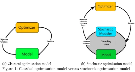
A sensible approach in this case would be to follow the model (Fig. 1b) proposed by (Painton and Diwekar, 1995), and to evaluate the objective functionW SDCseveral times and then consider the expected value as an estimator of the resulting distribution. However, even if the means are different, there is no guarantee the difference is not due to random chance.

The more general way to deal with this uncertainty about the statistical significance of the difference of expected values is to simply apply a standard statistical test in order to determine the significance level and decide whether or not to go ahead with the comparison. Another simpler approach, the one retained in fact, is to integrate into the scoring function a penalty factor that directly takes into account the variability of the distributions. This problem will specifically be addressed in more detail in Section 6.3.

6 Simulated Annealing

6.1 General Presentation

Simulated annealing is a stochastic combinatorial optimisation technique originally proposed by (Kirk-patrick et al., 1983). Given a functionf(θ)that takes a vector of discrete parametersθ, Simulated

(a) Classical optimisation model (b) Stochastic optimisation model

Figure 1: Classical optimisation model versus stochastic optimisation model

Annealing aims at finding the combination of parameter that maximises or minimises that function. (Kirkpatrick et al., 1983) draw a parallel between statistical mechanics and combinatorial optimisation and apply ideas from the Metropolis-Hastings algorithm (Metropolis et al., 1953) (simulation of the behaviour of many body systems) to combinatorial optimisation.

The principle of Simulated annealing is to first start from an initial configuration (combination) of the function parametersθ0as well as an initial temperatureT0. The initialθ0, is often chosen randomly, but putting an already good solution can accelerate the search.

Then, the algorithm iteratively applies a random change operatorRto the current configuration in order to obtain a modified configurationθ0=R(θ).

The value of the modified configurationf(θ0)is compared to the value of the current configurationf(θ), such that∆f=f(θ0)−f(θ). An acceptance functionP(∆f)is then used to determine whether to keep the current configuration or to accept the modified configuration.

In the original SA algorithm, the acceptance function is expressed using the Metropolis criterion and the Boltzmann distribution as shown in Equation 5.

P(∆f) =

(

1 if∆f<0

ex p€−∆f T

Š

otherwise (5)

With gradient descent or hill climbing search, only configuration that have a higher score are kept, while inferior configurations are systematically rejected. The problems with these approaches lies in the fact that complex functions often have many local minima and maxima, and the algorithm will likely converge on such a minimum or maximum.

Simulated Annealing, on the other hand, has a probability of accepting inferior configurations as a local minima/maxima escape strategy. The initial temperature is chosen so that at the beginning of the exploration, inferior configurations are almost always kept. After each iteration of the simulation, the temperature decreases and with it the probability to keep inferior configuration. As such, the algorithm starts with a wide and coarse exploration of the search space and then gradually converges on a fine grained exploration of a specific area around a minimum or maximum (hopefully close to the global minimum or maximum).

freezingtemperature or when the system is deemed to stabilize (usually a number of cycles during which improvements to the objective function are marginal or non-existent).

6.2 Cooling schedule and candidate generation

In SA, the way the temperature decreases is key to the performance of the algorithm. A logarithmic cooling schedule (Tn= T0

ln(n)) is theoretically sufficient in order to guarantee convergence (Ingber, 1996), however, it is too slow for many problems. A more common cooling schedule is geometricTn=T0·(α)n, where alpha is the cooling factor. However, on the one hand the slope of the cooling curve will be very steep even forαclose to one and on the other hand, the curve itself is convex. This means that the slope of the curve will get steep very fast, thus leading to a fast convergence at the cost of optimality. For this reason, (Ingber, 1996) proposes in his Adaptive Simulated Annealing algorithm to use an inverse exponential cooling schedule that will decrease quickly at the start and then slow down. Such a schedule corresponds much better to combinatorial optimisation algorithms, where we want to start with a broad search (accepting many inferior configurations) and then focus on a specific area of the search space. (Ingber, 1996) proposed the expression in equations 6 and 7, which we adopted for our implementation. Here,mandnare two scaling factors that can be used to tune the schedule for specific problems.

Tk=T0·ex p

−ci·k|1θ|

(6)

ci=m·ex p

−n D

(7)

Furthermore, the traditional SA, generates a new candidate configuration by uniformly selecting an index of the vector and by applying a random uniform change on the value, over the full range of possible values for that index. (Ingber, 1996) argues that once the system is colder, there is no point to explore the full range. Indeed, exploring an increasingly smaller neighbourhood as the temperature lowers and the systems converges on a specific area of the search space, allows an increase in computational efficiency while having no negative effects on the end result.

Equation 8 presents the probability distribution used for the candidate generation for each parameter, whereui∈U(0, 1)is a uniform random number between 0 and 1.

y=si gn

u−1₂

Tk

– 1+_Tk1

|2u−1|

−1 ™

(8)

From there, the new value of a parameterθ(i)_{ofθat iterationkcan be determined with the expression in} Equation 9 for a real parameter and Equation 10 for an integer parameter.

θ(i) k+1=θ(

i)

k +y(θmax(i) −θ( i)

min) (9)

θk(i+)1=θ(

i)

k +by(θmax(i) −θ( i)

min)c (10)

6.3 Handling uncertainty

As mentioned in Section 5, when dealing with an uncertain objective function, one needs to add an extra loop in the process, in order to generate samples from the evaluation of the objective functionf and then to use the expected value as a global objective function.

For a givenθ, we can build a list of samplesLs(θ) =SiN=0{f(θ)}and then consider a modified objective function that uses the expected value of the sample distribution:ΦE(θ) =xθ, wherexθ=N1·

P

6.4 Adaptive Penalty term

In order to deal with the variability of the distributions, (Painton and Diwekar, 1995) propose to add

to the expression ofΦE, a penalty factor based on the scaled standard deviationσθ=

qP

xi∈Ls(θ)(xi−xθ)2

N ,

weighted by a quantity that depends on the temperature. More specifically, their expression forΦEis:

ΦE(θ) =xθ+b(T)·

2_·σθ

p_N (11)

b(T) =_kb0T (12)

Whereb0is a small constant, k is a constant that represents the rate of increase ofb(T)andTthe temperature of the system.

Given that at the beginning, the temperature ishigh, the search is wide into the search space. Thus, accepting non-significant changes has little adverse effect, although it leads to less evaluation of the objective function (which is costly to compute in principle).

6.5 Significance testing

In this article, we take a slightly different approach, by integrating a standard statistical test directly in the metropolis criterion, and by usingΦEas only the expected value. Not only are such tests widely available

in existing libraries, additionally, we avoid the hassle of adding two more constants to the estimation algorithm.

Depending on the properties of the distribution, different tests may be applied. The most widely used test for significance is the unpaired two-sample student t-test. However three important pre-requisites must be met before the test can be applied.

The distributions of samples in the groups must be normal, the samples in the groups must be independent, and the variances of the groups must be equal. In the case of simulated annealing under uncertainty, there is no guarantee that the distributions all keep these properties. Thus, in order to use the t-test (Press et al., 1988), ot would be required to test the hypotheses for every new re-sampling of the objective function. This could be achieved by applying the Shapiro–Wilk (Shapiro and Wilk, 1965) test to test the normality assumption and Levene’s test (Levene, 1960) for the equality of variances.

In case the equality of variances criterion is not met, there is an alternative, Welch’s t-test (Welch, 1947) that does not make that assumption. However, if the distribution is not normal, there is no other choice but to apply a non-parametric test.

A much simpler alternative, is to directly apply a non-parametric significance test, such as the Mann–Whitney U unpaired test, as there are no assumption about the distribution of the samples. The only requirement is that the values are ordinal and not regularly paced.

6.5.1 Modified Metropolis criterion

Since the objective function returns a numerical value, the Mann–Whitney U can be applied directly in the metropolis criterion as such:

P(∆f) =

(

1 if∆PhiE<0 andpθ< α

e−∆PhiET otherwise (13)

threshold. If the p-value is below the threshold, then we reject the null-hypothesis and conclude that the distributions must be different.

For example withα=0.05 the null-hypothesis will be rejected if the probability of having a typeIerror is more that 95%: in other words,(1−p)>₍1−α₎.

The Mann–Whitney U (Mann and Whitney, 1947) is based on the comparison of the ranks of the samples within each group. The first step toward calculating the p-value is to group all the sample together, to sort them in ascending order, and to assign a rank to each value. From the respective ranks of the samples, can be computedRθ, is the sum of ranks forLs(θ)andRθ0the sum of ranks forLs(θ

0

). Here, the number of samples for both groups are always equal to N.

6.5.2 Computing the p-value

From the sum of ranks, the U statistic can be computed asU=min€Rθ−

N(N−1)

2 ;Rθ0−

N(N−1)

2 Š

=

minRθ;R_θ~0

−N(N−1)

2 .

For a sufficiently largeN, the U statistic is an approximation of the normal distribution, and after applying a standardization by calculating thezstatistic, the p-value can be retrieved from the probability density function of the normal distribution:

z=U−U

σU U=

N2

2 σU=

r

N2_(2N+1)

12 pθ=N(z,U,σU) =

1

p₂ π·σU

e−12

 z−U σU ‹2

(14)

Despite the apparent complexity of the process of calculating and testing the p-value, the Mann–Whitney U test is rather standard and available in many libraries for various programming languages, including Java that we used for our implementation.

7 Experimental protocol

The principle used for the evaluation of the variant of simulated annealing considered for the estimation of parameters in an uncertain setting, was to consider the Semeval 2007 Task 7 annotated corpus. We split the corpus into a training and a test set in order to evaluate the parameter search with the Ant Colony Algorithm for WSD originally proposed in (Schwab and Guillaume, 2011) and then further improved upon in (Schwab et al., 2012). Furthermore, we want to determine exactly how much data was necessary to obtain a good set of parameter values.

Normally, in order to obtain a reliable training and thus parameters, it would be necessary to have a somewhat larger test set and to split it into several parts by randomly aggregating words to perform ak−f oldcross validation. However, the Ant Colony algorithm is meant to work on a full text as it exploits its structure. Notably, the order of the words and the continuity of sentences are very important. Making cross-validation sets randomly would thus only create a very noisy training data. Even just picking sentences at random still compromises the global coherence of the solutions found, and thus the parameters.

This is why we only considered a training on successively larger portions of our training corpus. More specifically, the experiments were carried out with 6,12,18,24,30 and 36 sentences in order from the first sentences to the full text in multiples of 6.

The implementation of thisuncertainsimulated annealing, runs the ant colony algorithm and passes the results through to the scorer to obtain the F-score values. For the stochastic loop, for every new candidate configuration, the ant colony algorithm is systematically run 50 times in order to guarantee a sufficient level of statistical significance. The search was left to converge for each successive number of sentences and then, each resulting parameter values were tested over 100 executions of the ant colony algorithm on the test corpus in order to ascertain the quality of the parameters.

The results for each number of sentences are evaluated with relation to both classical lesk baseline and the baseline obtained with the parameters before the estimation (BL). We used standard statistical tests to guarantee the statistical significance of the comparisons.

8 Experiments and Results

8.1 Initial parameter for the simulated annealing estimator

Before starting the experiment, it is important to select the parameters of the simulated annealing-based algorithm we are using. In total there are 4 parameters.kst bthe number of cycles with no accepted new configurations before the system is considered to have converged.T0the initial temperature, andmand

n, the parameters of the cooling schedule. We are aware that the manual estimation of the parameters for the simulated annealing algorithm contradicts the general orientation of this paper, however one of the main reason simulated annealing was chosen is because its behaviour is well known and the parameters can be set heuristically quite effectively. Indeed a vast body of work covers the algorithm and can be used to guide the parameter estimation. The main idea is to use SA on algorithms with more complex and/or not so well understood parameter models. In fact, this process could be consider as a form of bootstrapping of sorts.

For the number of cycles before convergence, 20 is a good compromise between efficiency and optimality. As fornandm, we wanted to have a cooling schedule with the highest possible probability for subsequent iteration, while approaching 0 after 100 iterations. To this effect, after various experiments, we selected the valuesn=−3 andm=1.

0 0.1 0.2 0.3 0.4 0.5 0.6 0.7 0.8 0.9 1

0 0.02 0.04 0.06 0.08 0.1 0.12

P E O B A B IL IT Y O F A C C E P T A N C E INITIAL TEMPERATURE

(a) Choice of the initial temperature

159 13 17 21 25 29 33 37 41 45 49 53 57 61 65 69 73 77 81 85 89 93 0 0.1 0.2 0.3 0.4 0.5 0.6 0.7 0.8 0.9 CYCLES P R O B A B IL IT Y O F A C C E P T A N C E

(b) Cooling schedule acceptance probabilities

Figure 2: Classical optimisation model versus stochastic optimisation model

However, the most important parameter is the initial temperature, as it needs to be set to a certain level of probability of acceptance. Of course, since the probability of acceptance depends of the difference between successive scores, the first step toward selecting the initial temperature is to measure the average difference between successive scores. Therefore, it is necessary to run the algorithm while only sampling parameter configuration, without making any decisions about acceptance or convergence. Thus, we ran the algorithm this way and obtained an average F-score delta of0.57%with a standard deviation of 0.0047.

find the initial temperature, we can plot the graph of acceptance probability given the initial temperature (Figure 2a) by computinge−0.58Ti with various values ofTi. Given that T is in the same unit as the objective function, the value must be situated between 0 and 1. In the present case, the value ofTifor which

e−0.58Ti ₌0.8 is0.27. After the parameters have been set, it is possible to directly plot the cooling schedule in terms of the average acceptance probabilities (Figure 2b) by using Equation 6.

8.2 Analysis

For each text used as a training set, we applied the standard Shapiro-Wilks (Shapiro and Wilk, 1965) non-normality test and the Levene’s homoscedacity test (Levene, 1960) at aα=0.1 threshold, in order to verify the assumptions necessary to apply parametric statistical tests. For the results for Texts 1,2,3 the distributions resulting from each sentence led a to non-significant Shapiro Wilks, thus not allowing to reject the null hypothesis that the distributions are normal. Levene’s test was significant for all texts, meaning that the variances are homogeneous. However for texts 4 and 5, the Shapiro-Wilks test was significant, thus making us reject the null hypothesis that the distributions are normal.

Thus, for text 1,2 and 3 we applied a standard Anova test and found a p-value that is also significant at theα=0.01 level. Furthermore we carried out the Tukey pairwise test, which significant differences in mean between most groups unless otherwise specified.

For texts 4 and 5 we applied the non-parametric rank-based Kruskal-Wallis test (?), which is similar to ANOVA for situations where the distributions involved are not normal. For the non parametric pair-wise test, we applied a non-parametric variant of Tukey’s test, which the null hypothesis that "The probability of a sample frombbeing greater than a sample fromais superior to 0.5".

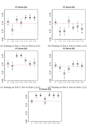
Table 3 and Figure 3a present the results for the first text as a training set in terms of value and in a graphical box plot representation.

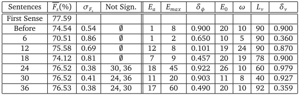
We can see for the first text in Table 3 and Figure 3a that with only 6 sentences, the results obtained after the estimations are worse that with the original parameters by 4.01%. With 12 and 18 sentences, the obtained results start to at the level of theBefore(BL on the graph) baseline. For 12 there is an improvement of 1.04% and for 18, a decrease of 0.42%. It appears that adding sentences is not necessarily positive, given that from 12 to 18 the results quality decreased.

Then, the results for 24, 30 and 36 are notably better than theBefore baselineby 1.98%, 1.98% and 1.99% and close, yet still below to the First Sense baseline with 1.07% to 0.8%. However, after 24 sentences, there aren’t any significant improvements by adding more sentences.

Sentences Fs(%) σFs Not Sign. Ea Emax δφ E0 ω Lv δv

First Sense 77.59

Before 74.54 0.54 ; 1 8 0.900 20 10 90 0.900 6 70.51 0.86 ; 1 2 0.650 10 5 90 0.360 12 75.58 0.69 ; 12 8 0.101 19 24 90 0.870 18 74.12 0.81 ; 7 9 0.457 20 19 78 0.900 24 76.52 0.38 30, 36 18 45 0.922 26 10 60 0.979 30 76.52 0.41 24, 36 11 20 0.903 11 8 40 0.927 36 76.53 0.38 24, 30 17 60 0.490 20 10 92 0.359

Table 3: Results in terms of the averageFscoreand its standard deviationσFsfor a given set of

parameter values. Unless specified, the pairwise Tukey HSD test is significant withα=0.01.

●

● ●

● ●

●

●

BL T1_S06T1_S12T1_S18T1_S24T1_S30T1_S36

F1 Score (%)

0.66

0.70

0.74

0.78

(a) Training on Text 1, Test on Texts 2,3,4,5

●

● ●

● ●

● ●

● ●

● ●

BL T2_30 T2_36 T2_S06T2_S12T2_S18T2_S24

F1 Score (%)

0.66

0.70

0.74

0.78

(b) Training on Text 2, Test on Texts 1,3,4,5

● ● ●

● ●

●

BL T3_S06T3_S12T3_S18T3_S24T3_S30T3_S36

F1 Score (%)

0.66

0.70

0.74

0.78

(c) Training on Text 3, Test on Texts 1,2,4,5

● ●

BL T4_S06T4_S12T4_S18T4_S24T4_S30T4_S36

F1 Score (%)

0.66

0.70

0.74

0.78

(d) Training on Text 4, Test on Texts 1,2,3,5

●

● ● ● ● ● ●

● ●

● ●

BL T5_S06T5_S12T5_S18T5_S24T5_S30T5_S36

F1 Score (%)

0.66

0.70

0.74

0.78

(e) Training on Text 5, Test on Texts 1,2,3,4

Sentences Fs(%) σFs Not Sign.

Lesk 73.64

Before 74.25 0.53 ;

6 74.86 0.74 ;

12 71.74 1.02 ;

18 72.27 0.65 ;

24 71.07 0.76 ;

30 69.81 0.53 36 36 70.06 0.70 30

(a) Results for Text 2 as a training corpus

Sentences Fs(%) σFs Not Sign.

Lesk 73.65

Before 74.54 0.57 30 6 73.15 0.64 ;

12 78.10 0.37 18 18 78.25 0.38 12 24 78.89 0.53 ;

30 74.18 0.54 BL 36 74.67 0.68 ; (b) Results for Text 3 as a training corpus

Sentences Fs(%) σFs Not Sign.

Lesk 72.80

Before 73.57 0.57 ;

6 72.18 0.73 ;

12 69.46 0.79 ;

18 71.75 0.74 ;

24 74.16 0.59 30 30 74.19 0.66 24 36 73.22 0.69 ; (c) Results for Text 4 as a training corpus

Sentences Fs(%) σFs Not Sign.

Lesk 75.85

Before 75.77 0.52 ;

6 76.60 0.37 12,24,30,36 12 78.68 0.33 24,30 18 76.86 0.69 ;

24 78.79 0.34 6,12,30 30 78.66 0.37 6,12,24,36 36 78.53 0.44 6,30

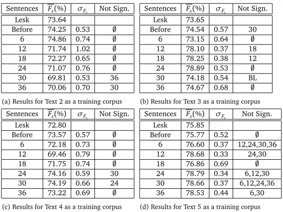
(d) Results for Text 5 as a training corpus

Table 4: Results in terms of the averageFscoreand its standard deviationσFsfor the parameters

found with each number of sentences of training data.

a profound effect. We can observe that for all three number of sentences 24, 30, 36, we systematically have:Ea<Emax,Ea≤E0and finallyδφ'δv. Given that for the number of sentences 24, 30 and 36 the

distribution are almost equal, we can hypothesise that there are to some degrees equivalences between some parameter value combinations.

We are also interested in the effect of the number of sentences by using the other texts of the corpus as training data. Furthermore we want to evaluate the fitness of certain types of texts for the purposes of parameter estimation for WSD. Tables 4a, 4b, 4c and 4d present the results for Texts 2,3,4,5 respectively as training sets. We will not, for these texts do a detailed analysis of the parameter values found, but will only look at the general trends with relation to the number of sentences and the properties of the texts. Figures 3b,3c,3d and 3e present box plots of the resulting score distributions for each text.

It is apparent that the quality of the parameter estimation widely depends on the nature of the texts used, as well as the quantity of data used for the training. For text 2, the results with any more than 6 sentences are all below the Lesk baseline, which could be indicative of a few general introductory sentences followed by very specific vocabulary. Text two is in fact an extract from the Wall Street Journal summarising a public scandal using very specific terms.

There are other cases, such as for text 3, where over fitting occurs very rapidly as the number of sentences increases. Such a behaviour could be explained by latter sentences of the text being domain specific and detrimental to the generality of the training. We observe a similar behaviour with text 4 towards the middle of the text. Text 3 is an extract from the wall street journal and is about a journalism convention, whereas Text 4 is a Wikipedia article about computer programming.

indicated by the non-significant differences. The results are about at the same distance above the Lesk baseline than in Text 1 with 24 sentences and above. Such a text would be very desirable for parameter training, as even little data is enough to obtain a very general training.

While it is not possible to make use of cross validation by taking random sentences, it may be a future possibility to take chunks of texts containing several sentences unified thematically or semantically for example and that have good training properties. Thus making a more formal cross-validation possible and allow to find the best combination of sentences for the purposes of parameter estimation with more systematic criteria.

9 Conclusions and Perspectives

We have presented and evaluated a variant of simulated annealing for uncertain cost functions. More specifically, we have adapted the work of (Painton and Diwekar, 1995) to use standard statistical tests, as well as integrated some elements of adaptivity inspired by (Ingber, 1996)’s Adaptive Simulated Annealing. We performed experiments on Semeval 2007 task 7 and found that the quality of the results from a given set of estimated parameters very much depend on the nature of the text. However, from the texts in our corpus it appears that very general texts with a diverse yet non domain specific lexicon are the best choice for the estimation of parameters. As exhibited for one of the texts, even very small training sets are sufficient to obtain good results granted the text has the right properties.

For future work concerning this parameter estimation approach, we are planning some more thorough experiments involving the other texts, as well parts of SemCor. Furthermore, there are many potential ways to improve the parameter search algorithm, notably through the integration of more adaptive elements from Adaptive Simulated Annealing. Furthermore, it may be beneficial to evaluate a variant where the statistical test is integrated in the objective function as a penalty term, like (Painton and Diwekar, 1995) propose with the standard deviation.

Furthermore, it would be very interesting to adapt our approach to perform joint optimisation of features and parameters as done in (Daelemans et al., 2003), even though the stochastic aspect would make it a much lengthier process in order to ensure statistically valid results.

Resources and programs

The implementations of both the parameter estimation and the Ant Colony Algorithm are both available online as Free Software under the GNU Lesser General Public License:https://forge.imag.fr/ projects/formica/. More information is available on the WSD page of our research group:http: //getalp.imag.fr/xwiki/bin/view/WSD/.

Funding

This research was funded by the French Ministry Research Allocation and by the Traouiero ANR project.

References

Bolhasani (2004). Parameter estimation of vehicle handling model using genetic algorithm. 11(1-2):121– 127.

Cowie, J., Guthrie, J., and Guthrie, L. (1992). Lexical disambiguation using simulated annealing. In

COLING ’92, pages 359–365, Nantes, France. ACL.

Daelemans, W., Hoste, V., Meulder, F. D., and Naudts, B. (2003). Combined optimization of feature selection and algorithm parameters in machine learning of language. InIn Proc of the 14th European Conference on Machine Learning, ECML 2003, pages 84–95, Cavtat-Dubrovnik, Croatia.

Workshop on the Evaluation of Systems for the Semantic Analysis of Text, pages 108–112, Barcelona, Spain. Association for Computational Linguistics.

Gelbukh, A., Sidorov, G., and Han, S.-Y. (2003). Evolutionary approach to natural language Word Sense Disambiguation through global coherence optimization.WSEAS Transactions on Communications, 1(2):11–19.

Goutte, C. and Gaussier, E. (2005). A probabilistic interpretation of precision, recall and f-score, with implication for evaluation. InECIR 27th European Conference on Information Retrieva, Santiago de Compostela, Spain.

Ingber, L. (1996). Adaptive simulated annealing (asa): Lessons learned. Control and Cybernetics, 25(1):33–54.

Katare, S., Bhan, A., Caruthers, J. M., Delgass, W. N., and Venkatasubramanian, V. (2004). A hybrid genetic algorithm for efficient parameter estimation of large kinetic models.Computers &amp; Chemical Engineering, 28(12):2569 – 2581.

Kay, S. M. (1993).Fundamentals of statistical signal processing: estimation theory. Prentice-Hall, Inc., Upper Saddle River, NJ, USA.

Kim, K.-J. and Diwekar, U. M. (2002). Efficient combinatorial optimization under uncertainty. 1. algorithmic development. 41(5):1276–1284.

Kirkpatrick, S., Gelatt, C. D., and Vecchi, M. P. (1983). Optimization by simulated annealing.Science, 220(4598):671–680.

Lee, Y. H., Park, S. K., and Chang, D.-E. (2006). Parameter estimation using the genetic algorithm and its impact on quantitative precipitation forecast.Annales Geophysicae, 24:3185–3189.

Levene, H. (1960). Robust tests for equality of variances. InIngram Olkin, Harold Hotelling, et alia., pages 278–292. Stanford University Press.

Mann, H. B. and Whitney, D. R. (1947). On a Test of Whether one of Two Random Variables is Stochastically Larger than the Other.The Annals of Mathematical Statistics, 18(1):50–60.

Metropolis, N., Rosenbluth, A. W., Rosenbluth, M. N., Teller, A. H., and Teller, E. (1953). Equation of state calculations by fast computing machines.The Journal of Chemical Physics, 21(6):1087–1092. Painton, L. and Diwekar, U. (1995). Stochastic annealing for synthesis under uncertainty.European Journal of Operational Research, 83(3):489 – 502.

Pan, Z., Chen, Y., Kang, L., and Zhang, Y. (1995). Parameter estimation by genetic algorithms for nonlinear regression. Inin G.Z.Liu (Ed.), Optimization Techniques and Applications, Proceedings of International Conference on Optimization Technique and Applications ’95, pages 946–953.

Paterakis, E., Petridis, V., and Kehagias, A. (1998). Genetic algorithm in parameter estimation of nonlinear dynamic systems. InProceedings of the 5th International Conference on Parallel Problem Solving from Nature, PPSN V, pages 1008–1017, London, UK, UK. Springer-Verlag.

Press, W. H., Flannery, B. P., Teukolsky, S. A., and Vetterling, W. T. (1988).Numerical recipes in C: the art of scientific computing. Cambridge University Press, New York, NY, USA.

Schwab, D., Goulian, J., Tchechmedjiev, A., and Blanchon, H. (2012). Ant colony algorithm for the unsupervised word sense disambiguation of texts: Comparison and evaluation. To be published. Schwab, D. and Guillaume, N. (2011). A global ant colony algorithm for word sense disambiguation based on semantic relatedness. InHighlights in Practical Applications of Agents and Multiagent Systems, volume 89 ofAdvances in Intelligent and Soft Computing, pages 257–264. Springer Berlin/Heidelberg. Shapiro, S. S. and Wilk, M. B. (1965). An analysis of variance test for normality (complete samples).

Sharman, K. and McClurkin, G. (1989). Genetic algorithms for maximum likelihood parameter estimation. InAcoustics, Speech, and Signal Processing, 1989. ICASSP-89., 1989 International Conference on, pages 2716 –2719 vol.4.

Veronis, J. and Ide, N. M. (1990). Word sense disambiguation with very large neural networks extracted from machine readable dictionaries. InProceedings of the 13th conference on Computational linguistics -Volume 2, COLING ’90, pages 389–394, Stroudsburg, PA, USA. Association for Computational Linguistics. Welch, B. L. (1947). The Generalization of ‘Student’s’ Problem when Several Different Population Variances are Involved.Biometrika, 34(1/2):28–35.