LSTM autoencoders for dialect analysis
Taraka Rama Department of Linguistics University of Tübingen, Germany
taraka-rama.kasicheyanula @uni-tuebingen.de
Ça˘grı Çöltekin Department of Linguistics University of Tübingen, Germany
ccoltekin
@sfs.uni-tuebingen.de
Abstract
Computational approaches for dialectometry employed Levenshtein distance to compute an ag-gregate similarity between two dialects belonging to a single language group. In this paper, we apply a sequence-to-sequence autoencoder to learn a deep representation for words that can be used for meaningful comparison across dialects. In contrast to the alignment-based methods, our method does not require explicit alignments. We apply our architectures to three different datasets and show that the learned representations indicate highly similar results with the anal-yses based on Levenshtein distance and capture the traditional dialectal differences shown by dialectologists.
1 Introduction
This paper proposes a new technique based on state-of-the-art machine learning methods for analyzing dialectal variation. The computational/quantitative study of dialects,dialectometry, has been a fruitful approach for studying linguistic variation based on geographical or social factors (Goebl, 1993; Ner-bonne, 2009). A typical dialectometric analysis of a group of dialects involve calculating differences between pronunciations of a number of items (words or phrases) as spoken in a number of sites (ge-ographical location, or another unit of variation of interest). Once a difference metric is defined for individual items, item-by-item differences are aggregated to obtain site-by-site differences which form the basis of further analysis and visualizations of the linguistic variation based on popular computational methods such as clustering or dimensionality reduction. One of the key mechanisms for this type of anal-ysis is the way item-by-item differences are calculated. These distances are often based on Levenshtein distance between two phonetically transcribed variants of the same item (Heeringa, 2004). Levenshtein distance is often improved by weighting the distances based on pointwise mutual information (PMI) of the aligned phonemes (Wieling et al., 2009; Prokic, 2010).
In this paper we propose an alternative way for calculating the distances between two phoneme se-quences using unsupervised (or self supervised) deep learning methods, namely Long Short Term Mem-ory (LSTM) autoencoders (see Section 2 for details). The model is trained for predicting every pronun-ciation in the data using the pronunpronun-ciation itself as the sole predictor. Since the internal representation of the autoencoder is limited, it is forced to learn compact representations of words that are useful for recon-struction of the input. The resulting internal representations,embeddings, are (dense) multi-dimensional vectors in a space where similar pronunciations are expected to lie in proximity of each other. Then, we use the distances between these embedding vectors as the differences between the alternative pronun-ciations. Since the distanced calculated in this manner are proper distances in an Euclidean space, the usual methods of clustering or multi-dimensional scaling can be applied without further transformations or normalizations.
There are a number of advantages of the proposed model in comparison to methods based on Lev-enshtein distance. First of all, proposed method does not need explicit alignments. While learning to reconstruct the pronunciations, the model discovers a representation that places phonetically similar This work is licenced under a Creative Commons Attribution 4.0 International License. License details: http:// creativecommons.org/licenses/by/4.0/
r o U z
r o U z
Embeddings
Encoder
[image:2.595.150.456.64.187.2]Decoder
Figure 1: The demonstration of LSTM autoencoder using an example pronunciation [roUz] (rose). The
encoder part represents the whole sequence as a fixed-size embedding vector, which is converted to the same sequence by the decoder.
variants together. However, unlike other alternatives, the present method does not need pairs of pronun-ciations of the same item. Another advantage of the model is its ability to discover potential non-linear and long-distance dependencies within words. The use of (deep) neural networks allow non-linear com-binations of the input features, where LSTMs are particularly designed for learning relationships at a distance within a sequence. The model can learn properties of input that depend on non-contiguous long-distance context features (e.g., as in vowel harmony) and it can also learn to combine features in a non-linear non-additive way, (e.g., when the effect of vowel harmony is canceled in presence of other contextual features).
The rest of the paper is organized as follows. In section 2, we describe our model and the reasons for the development and employment of such a model. In section 3, we discuss our experimental settings and the results of our experiments. We discuss our results in section 4. We conclude the paper in section 5.
2 Model
As mentioned in the previous section, the computational approaches in dialectometry compare words using Levenshtein distance and aggregate the Levenshtein distance across concepts to project the distance matrix on a map. In this paper, we propose the use of autoencoders (Hinton and Salakhutdinov, 2006) based on Long Short Term Memory neural networks (LSTMs) (Hochreiter and Schmidhuber, 1997) for capturing long distance relationships between phonemes in a word. Originally, autoencoders were used to reduce the dimensionality of images and documents (Hinton and Salakhutdinov, 2006). Hinton and Salakhutdinov (2006) show that the deep fully connected autoencoders, when applied to documents, learn a dense representation that separates documents into their respective groups in two dimensional space.
Unlike standard deep learning techniques which learn the neural network weights for the purpose of classification, autoencoders do not require any output label and learn to reconstruct the input. Typical autoencoders feature a hour-glass architecture where the lower half of the hour glass architecture is used for learning a hidden representation whereas, the upper half of the architecture (a mirror of the lower half) learns to reconstruct the input through back-propagation. The learned intermediate representation of each word is a concise representation its pronunciation. The network is forced to use information-dense representations (by removing or reducing redundant features in the input) to be able to construct the original pronunciation. These representations, which are similar to well-known word embeddings (Mikolov et al., 2013; Pennington et al., 2014) in spirit, can then be used for many tasks. In our case, we use the similarities between these internal vector representations for quantifying the similarities of alternative pronunciations. Although the lengths of the pronunciations vary, the embedding representa-tions are fixed. Hence each pronunciation is mapped to a low dimensional space,Rk, such that similar
pronunciations are mapped to close proximity of each other.
of a word. The LSTM autoencoder has two parts: encoder and decoder. The encoder part transforms the input sequence(x1, . . . xT)to a hidden representationh∈Rkwhere,kis a predetermined
dimensional-ity ofh. The decoder is another LSTM layer of lengthT. Theht=hrepresentation at each time stept
is fed to a softmax function ( ehtj P
kehtk) that outputs axˆt ∈R
|P|length probability vector whereP is the set of phonemes in the language or the language group under investigation.
In this paper, we represent a word as a sequence of 1-hot-|P|vectors and use the categorical cross-entropy function (−Ptxtlog( ˆxt) + (1−xt)log(1−xˆt)) wherextis a 1-hot vector andxˆtis the output
of the softmax function at timestept) to learn both the encoder and decoder LSTM’s parameters. We tested with both unidirectional (−→h) and bidirectional encoder representations in our experiments. The bidirectional encoder consists of a bidirectional LSTM where the input word is scanned in both directions to compute a concatenated −→h L←h−which is then fed to a decoder LSTM layer for recon-structing the input word.
The model we use is different from theseq2seqmodel of Sutskever et al. (2014) in that theseq2seq
model supplies the hidden representation of the input sequence to predict the first symbol in a target sequence and then uses the predicted target symbol as an input to the LSTM layer to predict the current symbol. Our architecture, is simpler than theseq2seqmodel due to the following reasons:
1. Unlikeseq2seq, we work with dialects of a single language which do not require explicit language modeling that features in cross-language sequence learning models.
2. Our model is essentially a sequence labeling model that learns a dense intermediate representation which is then used to predict the input sequence. Moreover, unlike neural machine translation, the source and target sequences are identical, hence, have the same length in our case.
The motivation behind the use of autoencoders is that a single autoencoder network for all the site data would learn to represent similar words with similar vectors. Unlike Levenshtein distance, the LSTM autoencoders can learn to remember and forget the long distance dependencies in a word. The general idea is that similar words tend to have similar representations and a higher cosine similarity. By training a single autoencoder for the whole language group, we intend to derive a generalized across-concept representation for the whole language group.
Once the network is trained, we use the similarities or differences between internal representations of different pronunciations to determine similarities or differences between alternative pronunciations. Since embeddings are vectors in an Euclidean space, similarity can easily be computed using cosine of the angle between these vectors. Then, we use Gabmap (Nerbonne et al., 2011; Leinonen et al., 2016) for analyzing the distances and visualizing the geographic variation on maps. Since Gabmap requires a site-site distance matrix to visualize the linguistic differences between sites, we convert the cosine similarity to a distance score by shifting a similarity score by 1.0 followed by a division by 2.0. The shifted similarity score is then subtracted from 1.0 to yield a distance score. The distance for a site pair is obtained by averaging the word distances across concepts. In case of synonyms, we pick the first word for each concept.
3 Experiments and Results
3.1 Data
We test the system with data from three different languages, English, Dutch and German. The English data comes from Linguistic Atlas of the Middle and South Atlantic States (LAMSAS; Kretzschmar (1993)) The data includes 154 items from 67 sites in Pennsylvania. The data is obtained from Gabmap site,1and described in Nerbonne et al. (2011).
The Dutch dialect data is form the Goeman-Taeldeman-Van Reenen Project (Goeman and Taelde-man, 1996) which comprises 1876 items collected from more than 600 locations in the Netherlands and
Flanders between 1979–1996. It consists of inflected and uninflected words, word groups and short sen-tences. The data used in this paper is a subset of the GTRP data set and consist of the pronunciations of 562 words collected at 613 locations. It includes only single word items that show phonetic variation.
German dialect data comes from the project ‘Kleiner Deutscher Lautatlas – Phonetik’ at the ‘Forschungszentrum Deutscher Sprachatlas’ in Marburg. The data was recorded and transcribed in the late 1970s and early 1990s (Göschel, 1992). In this study, we the data from Proki´c et al. (2012) which is a subset of the data that consists of the transcriptions of 40 words that are present at all or almost all 186 locations evenly distributed over Germany.
3.2 Experimental setup
In our experiments, we limitT, the length of the sequence processed by the LSTM, to10for Dutch and German dialect datasets and20 for Pennsylvanian dataset. We trained our autoencoder network for 20 epochs on each dataset and then used the encoder to predict a hidden representation of length8for each dataset. We used the continuous vector representation to compute the similarities between words. We used a batch size of32and theAdadeltaoptimizer (Zeiler, 2012) to train our neural networks. All our experiments were performed using Keras (Chollet, 2015) and Tensorflow (Abadi et al., 2016).
3.3 Results
In this section we first present an example visualization of the learned word representations in the hidden dimensions of LSTM autoencoders. To present the model’s success in capturing geographical variation, we present visualizations from three different linguistic areas. The maps and the MDS plots in this section were obtained using Gabmap.
3.4 Similarities in the embedding space
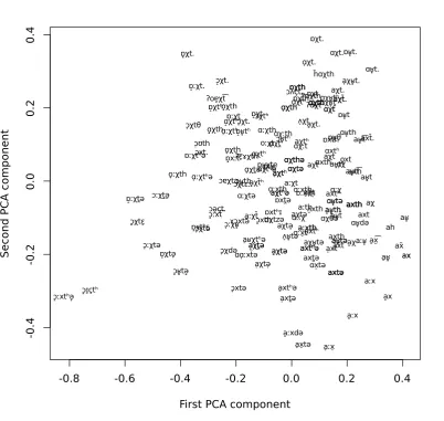
Figure 2 presents first two dimensions of the PCA projection of the embedding vectors for alternative pronunciations of German wordacht‘eight’. As the figure shows, similar pronunciations are closer to the each other in this projection.
Although the representation in Figure 2 show that similar pronunciations are close to each other in this projection, we note that the vector representation are already dense. As a result, unlike many data sets with lots of redundancy, the first two PCA components does not contain most of the information present in all 8 dimensions used in this experiment. The first two PCA component above only explains 50% of the total variation. Hence, half of the variation is not visible in this graph, and some of the similarities or differences shown in the figure may be not be representative of their actual similarities or differences. However, as the analyses we present next confirm, the distances between these representations in the unreduced 8 dimensional space captures the geographical variation well.
3.4.1 Pennsylvanian dialects
An interesting dialect region often analyzed in the literature is the Pennsylvanian dialects. We visualize the distances between sites by reducing the distances using MDS and projecting it on a map for both uni-directional and biuni-directional LSTM autoencoders and for a typical Levenshtein distance analysis (using Gabmap with default settings). Figure 3 presents a shaded map where shades represent the first MDS di-mension. The reduction to a single dimension preserves 88%, 90% and 96% of the original distances for unidirectional LSTM, Levenshtein distance and bidirectional LSTM, respectively. The results are again similar to the earlier analyses (Nerbonne et al., 2011). Here all analyses indicate a sharp distinction between the ‘Pennsylvanian Dutch’ area and the rest of Pennsylvania. This distinction is even sharper in the maps produced by the LSTM autoencoders. However, within each group distances indicated by the LSTM autoencoders are smaller, hence, transitions are smoother. The famous ‘Route 40’ boundary is also visible in all analyses, however, it is sharper in the classical Levenshtein distances in comparison to the LSTM autoencoders.
-0.8 -0.6 -0.4 -0.2 0.0 0.2 0.4
-0.4
-0.2
0.0
0.2
0.4
First PCA component
Second PCA component
ɑχtʰə̹
ɔ̠̜χtɛ̠
a̠xtʰ ɑχth
a̠χt̪ə ɒ̝χtʰ
ax̆ ɑχt
axt̪ə ɔ̞ʁ̥tə̝
oxt
a̠ʁ̥th
aʁ̥ ɒχth
ɑ̝̹χth
ɑːχ
a̠χtə̹
ɔ̝ːxtʰə̝
ɑxtʰ
aχtʰə
axth
ah
ɑχtzə
ɔ̝ɪ̠çtʰ
ɑ̠χt̪
axtə ɒχt
ɑʁ̥tə ɒ̝χt
ɑːxth
ɑ̝χtʰ
ax
ʌ̞ʁ̥tə
ɑʁ̥t.
ɔʁ̥tʰ
axt͡ ɔ̞χt.
a̠χtə ɒ̝̜χt.
axt
ɒxtʰɪ
ɑːx̠t
ɒ̝ːχt.
ɒʁ̥t.
ɒχt�h�
ax̠th
ɑ̹χt.
a̠χʁ̥tə
a̠xt� ɑ̞χtʰ
ax
ɑːχtə
aʁ̥tə
aʁ̥t
ɔχtɛː
oːχt
ɒ̝χtə̞
ɔ̞ʁ̥th
a̹χʁ̥t.
o̞ːχth
ɔχtʰ
ɑχtə ɑ̹ːχtʰ
ɑχtʰ
aχtə̹
aːʁ̥
aχt.
ɑχt
aχ
h� ɑχth
ɒ̝xtʰɛ̠
ɔ̞xtə
aʁ̥tʰ
axth
ɑʁ̥tə
ɒ̝χth ɑχth
aːxth
a̠xt̪ə ɤɔxtə̃
ɒχθ
ʔɛ̠ɤχth
ɑχth
a̠χ ɑχthə
ɔ̞̜xt.
ɒxt̪ə
a̠x̤͡
aʁ̥t͡ ɔ̜χtθ
aːχt
axtʰ
a̠x̆t
ɔ̞χdə
aːx
ɑχːth
ɔʌçt.
ɑx̠tə ɒːxʔn̩
aχt�.
ɑχth
ɔ̞xth
ɒ̝ːχt̪ə
ɑ̹χth
aχtə ɔ̝χt.
a̠ːxdə ɒːχt̪
a̠χtʰ ɒχth
ɒ̜ːχ
ɑχth
a̠χt
ɒʁ̥χte̝
ɑχʁ̥tʰ
axt�.
a̠ːχt�
axth
ɑχʁ̥t̪
ɑ̹χ
a̠χtə
a̠ʁχtʰə
axth
ɒxth
ɑɑ̹ːxt�ə
aχt
ɔːχt̪ə̤
ɔ̞ːχtə
ɑ̹χt̪ə
ɑχthə ɑχːt
ɑːːχ
a̠ːx̠ ɒ̝xːt͡
ɑʁ̥th
a̠ʁ̥ ɒχth
ɑχtə ɒχt.
aʁ̥th
ɑʁ̥də
axtə
aχtʰ
ɔ̞ːxt͡
a̠ːx aːxth
a̠x̠tə
a̠̹χt�ʰ
aːth
a̠x
ɑ̹ːχtʰə
a̠xtʰə
aχtʰə ɑχth
ɑχθə
a̠χt̪ə axtaxtʰəʰə ɔ̜ʊth
a̠χt.
ɑ̹χth
ʔɑχth aχt�.
aʁ̥tə ɒ̝ʁ̥tʰ
a̠χtʰ
ɒʁ̥t
ɔə̞çt.
ɔ̞ːχʁ̥
ɑ̹xth
a̠ʁ̥t� ɑːχth
a̠ʁ̥th o̞χth
ɔɐχtə
ɑχt.
ɑ̹ːxth a χt
ʔɑχt�
ʌ̞xth
ʔoɐ̠χt͡
axtə ɔ̞χtə
ʌ̹χt
[image:5.595.97.500.86.467.2]ɒːχtʰə
Figure 2: PCA analysis of the dense representation of the German wordacht‘eight’.
this area and the rest in the LSTM autoencoder output but not as strong in the results with Levenshtein differences.
3.4.2 Dutch dialects
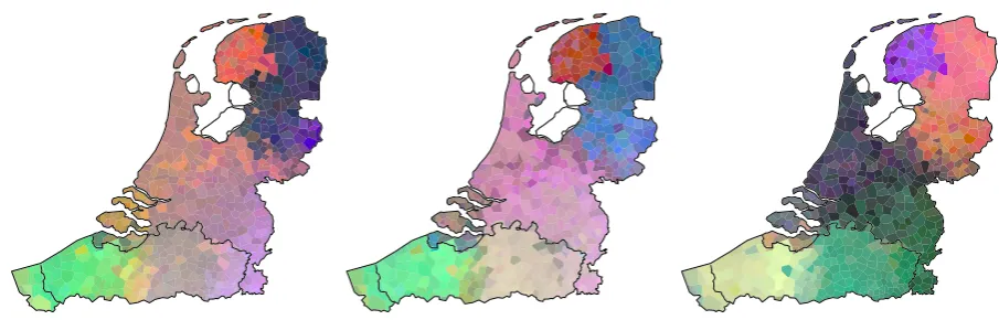
Figure 5 presents the multi-dimensional scaling (MDS) applied to distances based on both unidirectional and bidirectional LSTM autoencoder in comparison to classical Levenshtein distance. The distances in the first three dimensions of MDS are mapped to RGB color space. The correlation between the dis-tances in the first three dimensions and the disdis-tances in the unreduced space are 89% for Levenshtein and unidirectional LSTM autoencoder, and 94% for the bidirectional LSTM autoencoder. All methods yield similar results which are also in-line with previous research (Wieling et al., 2007). The colors indi-cate different groups for Frisian (north west), Low Saxon (Groningen and Overijsel, north east), Dutch Franconian varieties (middle, which seem to show gradual changes from North Holland to Limburg), and Belgian Brabant (south east) and West Flanders (south west).
Figure 3: MDS analysis of Pennsylvanian dialects. The shades represent only the first MDS dimension. The distances are based on distances of bidirectional recurrent autoencoder representations (left), unidi-rectional (middle) and aggregate Levenshtein distance (right). Note that the colors are arbitrary, only the differences (not the values) are meaningful.
Figure 4: First two MDS dimensions plotted against each other for the Pennsylvania data. Distances are based on concatenated bidirectional LSTM autoencoder representation (left), unidirectional LSTM encoder (middle) and classical aggregate Levenshtein difference (right).
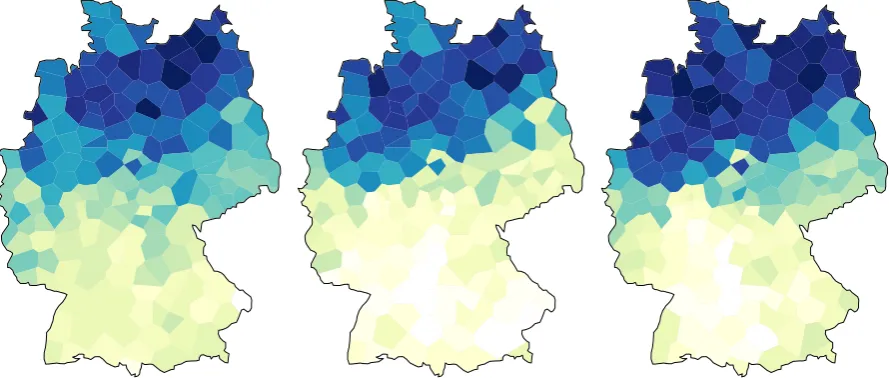
[image:6.595.70.523.520.665.2]Figure 6: MDS analysis of the German dialects. The shades represent only the first MDS dimension. The distances are based on distances of bidirectional recurrent autoencoder representations (left), unidi-rectional (middle) and aggregate Levenshtein distance (right).
3.4.3 Dialects of Germany
Figure 6 presents similar analyses for dialects of Germany. Similar to Pennsylvania data, we only vi-sualize the first MDS dimension, with correlations with the original distances 62%, 68% and 70% for unidirectional LSTM, bidirectional LSTM and Levenshtein distances, respectively. The MDS maps of the German dialects show the traditional two-way classification along the North-South dimension. The unidirectional autoencoder shows a higher transition boundary as compared to the bidirectional autoen-coder. This seems to be in line with the observation that autoencoders represent a smoother transition in comparison to Levenshtein distance.
4 Discussion
The results of the above visualization show that sequence-to-sequence autoencoders capture similar in-formation to that of pair-wise Levenshtein distance. The autoencoders only require list of words in a uniformly transcribed IPA format for learning the dense representation as compared to the pair-wise ap-proach adopted in Levenshtein distance. We hypothesize that the dense representation of a word causes the smooth transition effect that is absent from the maps of Levenshtein distance. Our experiments suggest that the autoencoders require few thousands of words to train and the visualizations of the site distances correlate well with the traditional dialectological knowledge. An advantage of autoencoders is that they do not require explicit alignment and can train to reconstruct the input.
5 Conclusions
In this paper, we introduced the use of LSTM autoencoders for the purpose of visualizing the shifts in dialects for three language groups. Our results suggest that LSTM autoencoders can be used for visu-alizing the transitions across dialect boundaries. The visualizations from autoencoders correlate highly with the visualization produced with the standard Levenshtein distance (used widely in dialectometry). LSTM autoencoders do not require explicit alignment or a concept based weighting for learning realis-tic distances between dialect groups. In the future, we aim to apply the LSTM autoencoders to speech recordings of dialects for the purpose of identifying dialect boundaries.
Acknowledgements
References
Martín Abadi, Ashish Agarwal, Paul Barham, Eugene Brevdo, Zhifeng Chen, Craig Citro, Greg S Corrado, Andy Davis, Jeffrey Dean, Matthieu Devin, et al. 2016. Tensorflow: Large-scale machine learning on heterogeneous distributed systems. arXiv preprint arXiv:1603.04467.
François Chollet. 2015. Keras: Deep learning library for theano and tensorflow.
Hans Goebl, 1993. Dialectometry: a short overview of the principles and practice of quantitative classification of linguistic atlas data, pages 277–315. Springer Science & Business Media.
Antonie Goeman and Johan Taeldeman. 1996. Fonologie en morfologie van de nederlandse dialecten. een nieuwe materiaalverzameling en twee nieuwe atlasprojecten. Taal en Tongval, 48:38–59.
Joachim Göschel. 1992. Das Forschungsinstitut für Deutsche Sprache “Deutscher Sprachatlas”. Wis-senschaftlicher Bericht, Das Forschungsinstitut für Deutsche Sprache, Marburg.
Wilbert Jan Heeringa. 2004. Measuring dialect pronunciation differences using Levenshtein distance. Ph.D. thesis, University of Groningen.
Geoffrey E Hinton and Ruslan R Salakhutdinov. 2006. Reducing the dimensionality of data with neural networks. Science, 313(5786):504–507.
Sepp Hochreiter and Jürgen Schmidhuber. 1997. Long short-term memory. Neural computation, 9(8):1735–1780. William A Kretzschmar. 1993. Handbook of the linguistic atlas of the Middle and South Atlantic States.
Univer-sity of Chicago Press.
Therese Leinonen, Ça˘grı Çöltekin, and John Nerbonne. 2016. Using Gabmap.Lingua, 178:71–83.
Tomas Mikolov, Ilya Sutskever, Kai Chen, Greg S Corrado, and Jeff Dean. 2013. Distributed representations of words and phrases and their compositionality. In Advances in neural information processing systems, pages 3111–3119.
John Nerbonne, Rinke Colen, Charlotte Gooskens, Peter Kleiweg, and Therese Leinonen. 2011. Gabmap – a web application for dialectology. Dialectologia, Special Issue II:65–89.
John Nerbonne. 2009. Data-driven dialectology. Language and Linguistics Compass, 3(1):175–198.
Jeffrey Pennington, Richard Socher, and Christopher D Manning. 2014. Glove: Global vectors for word represen-tation. InEMNLP, volume 14, pages 1532–1543.
Jelena Proki´c, Ça˘grı Çöltekin, and John Nerbonne. 2012. Detecting shibboleths. InProceedings of the EACL 2012 Joint Workshop of LINGVIS & UNCLH, pages 72–80. Association for Computational Linguistics. Jelena Prokic. 2010. Families and resemblances.
Ilya Sutskever, Oriol Vinyals, and Quoc V Le. 2014. Sequence to sequence learning with neural networks. In Advances in neural information processing systems, pages 3104–3112.
Martijn Wieling, Wilbert Heeringa, and John Nerbonne. 2007. An aggregate analysis of pronunciation in the goeman-taeldeman-van reenen-project data. Taal en Tongval, 59(1):84–116.
Martijn Wieling, Jelena Proki´c, and John Nerbonne. 2009. Evaluating the pairwise string alignment of pronuncia-tions. InProceedings of the EACL 2009 workshop on language technology and resources for cultural heritage, social sciences, humanities, and education, pages 26–34.
![Figure 1: The demonstration of LSTM autoencoder using an example pronunciation [roUz] (rose)](https://thumb-us.123doks.com/thumbv2/123dok_us/1487191.688731/2.595.150.456.64.187/figure-demonstration-lstm-autoencoder-using-example-pronunciation-rouz.webp)