doi:10.4236/jcc.2013.11001 Published Online February 2013 (http://www.scirp.org/journal/jcc)
Numerical Methods for Solving Turbulent Flows by Using
Parallel Technologies
Alibek Issakhov
Department Mechanics and Mathematics, al-Farabi Kazakh National University, Almaty, Kazakhstan Email: [email protected]
Received 2013
ABSTRACT
Parallel implementation of algorithm of numerical solution of Navier-Stokes equations for large eddy simulation (LES) of turbulence is presented in this research. The Dynamic Smagorinsky model is applied for sub-grid simulation of tur-bulence. The numerical algorithm was worked out using a scheme of splitting on physical parameters. At the first stage it is supposed that carrying over movement amount takes place only due to convection and diffusion. Intermediate field of velocity is determined by method of fractional steps by using Thomas algorithm (tridiaginal matrix algorithm). At the second stage found intermediate field of velocity is used for determination of the field of pressure. Three dimensional Poisson equation for the field of pressure is solved using upper relaxation method. Moreover various ways of geome-trical decomposition for parallel numerical solution of three dimensional Poisson equations are investigated.
Keywords: Domain Decomposition; Parallel Computations; Dynamic Smagorinsky Model; LES Approach
1.
Introduction
Most flows occurring in nature and in engineering appli-cations are turbulent. Turbulent flow is a fluid motion that possesses complex and seemingly random structure at some macroscopic scale of dynamical importance. The most important physical consequence of turbulence is the enhancement of transport processes. In turbulent flow, momentum, energy and particle transport rates greatly exceed the corresponding molecular transport rates. Turbulent flow exhibit much more small-scale structure than their non-turbulent counterparts. In fact, this small-scale structure is correlated with enhanced turbu-lent transport phenomena. Small-scale structure itself is evidence of enhanced transport in the sense that small scale develop from the degradation of large-scale excita-tions and are maintained by energy transport from one scale to another. Another important characteristic of tur-bulent flows is their apparent randomness and instability to small perturbations. Currently, there are three basic and commonly used approaches for simulation of turbu-lent flows. First approach is direct numerical simulation (DNS) which applies to solve Navier – Stokes equations, resolving all the scales of motion, with initial and boun-dary conditions appropriate to the considered flow. Each simulation produces a single realization of the flow. The DNS approach was infeasible until the 1970s when
Navi-er–Stokes equations (or RANS equations) are time-averaged equations of motion for fluid flow. The idea behind the equations is Reynolds decomposition, whereby an instantaneous quantity is decomposed into its time-averaged and fluctuating quantities, an idea was first proposed by Osborne Reynolds. The RANS equa-tions are primarily used to describe turbulent flows. These equations can be used with approximations based on knowledge of the properties of flow turbulence to give approximate time-averaged solutions to the Navi-er–Stokes equations.
2.
Mathematical Model
Under the assumption of incompressible flow, the di-mensionless governing equations are as follows [1,2,7]:
j ij j i j i j i j i
x
x
u
x
x
p
x
u
u
t
u
∂
∂
−
∂
∂
∂
∂
+
∂
∂
−
=
∂
∂
+
∂
∂
τ
Re
1
(1) ). 3 , 2 , 1 ( 0 = = ∂ ∂ i x u j j (2)where
τ
ij=
u
iu
j−
u
iu
jThe solution of spread of flow in three dimensional
areas were considered in this work.
u
i velocity, prepresents the total pressure. The Reynolds number is defined as
Re
=
DV
/
ν
(ν
dynamic viscosity). Fur-thermore Cartesian coordinate system is employed, in which z is stream wise direction, x, y are in the lateral directions.As for constructing model of turbulence we used dy-namic model of Smagorinsky, the following is the un-derlying principle of the dynamic model for extracting information concerning a given eddy-viscosity model via a double filtering in physical space. It is worth to admit that the most of the historical developments have been done with Smagorinsky’s model [6,9]
ij sgs kk
ij
ij
δ
τ
ν
s
τ
2
3
1
=
−
−
(3)
≠
=
=
j
i
j
i
ij,
0
,
1
δ
Kroneker symbolwhere
ν
sgs=
(
C
s∆
)
22
s
ijs
ij ,
∂
∂
+
∂
∂
=
i j j i ijx
u
x
u
s
2
1
,
∆
=
(
∆
x
∆
y
∆
z
)
1/3 (4)4 / 3 2 3 1 − = k s C C
π
,C
s=0.18 for a Kolmogorov con-stant of 1,4.But the dynamic procedure applies in fact to the types of eddy viscosities such as those used in the struc-ture-function model.
We start with regular LES corresponding to a “bar-filter” of width
∆
x
, an operator associating anfunction
f
(
x
,
t
)
. Then we define a second “test filter”tilde of large width
2
∆
x
associating(
,
)
~
t
x
f
−
. So let us first apply this filter product to the Navier-Stokes
equa-tion. The subgrid-scale tensor of the field
~
i
u
is ob-tained from equation (4) with the replacement of the fil-ter bar by the double filfil-ter and tilde filfil-ter:~ ~ ~ j i j i
ij
=
u
u
−
u
u
τ
(5)~ ~ ~ j i j i
ij
u
u
u
u
l
=
−
(6)Now we apply the tilde filter to equation (4), which leads to ~ ~ ~ j i j i
ij
=
u
u
−
u
u
τ
(7)Adding equations (6) and (7) and using equation (5), we obtain
~
ij ij ij
l
=
τ
−
τ
Further we use Smagorinsky’s model expression for the subgrid stresses related to the bar filter and tilde-filter to get ~ ~ ~
2
3
1
ij kk ijij
−
δ
τ
=
−
C
A
τ
where
A
ij=
(∆
x
)
2S
S
ij ( 8 )We have to determine
τ
ij, the stress resulting fromthe filter product. This is again obtained using the Sma-gorinsky model, which yields
ij kk
ij
ij
2
CB
3
1
−
=
−
δ
τ
τ
where~ ~ 2 ) 2 ( ij
ij x SS
Subtracting (8) from (9) with the aid of Germano’s identity we get the following
~
2
2
3
1
ij ij
kk ij
ij
l
CB
C
A
l
−
δ
=
−
ij kk
ij
ij
l
CM
l
2
3
1
=
−
δ
where
~
ij ij
ij
B
A
M
=
−
( 1 0 )All the terms of equation (10) may now be determined
by means of
u
. Unfortunately, there are five indepen-dent equations for only one variable C, and thus the problem is over determined. The first solution waspro-posed by Germano to multiply (10) tensorially by
S
ijto get
ij ij
ij ij
S M
S l C
2 1 =
3.
Numerical Simulation
The numerical solution of system is built on the stag-gered grid with the usage of the compact scheme for convective terms and scheme against a stream of the second type [5].
The scheme of splitting on physical parameters is used for the solution of turbulence problem [9-12,14]:
I.
(
* *)
,
*
u
u
u
u
u
nn
∆
−
∇
−
=
−
ν
τ
II.
,
*
τ
u
p
∇
=
∆
III.
.
* 1
p
u
u
n+−
=
−∇
τ
The first stage is solved by fractional step method in combination of Thomas algorithm (tridiaginal matrix algorithm) [8, 11,13].
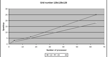
Three dimensional Poisson equation for pressure field using an over - relaxation method is handled at the second stage. Three dimensional Poisson equation is parallelized by using various geometrical decomposition (1D, 2D and 3D). Geometric decomposition of the grid area is selected as the basic approach of parallelization. In this case, there are three different ways of sharing the values of the grid function on the compute nodes one-dimensional, two-dimensional and three-dimensional of the grid computing nodes [3,4].
After a stage of decomposition, when performed on separate data blocks for the construction of a parallel algorithm, we proceed to relation between the blocks, the
calculations which will be run parallel. Because of we used an explicit difference scheme for computing the next approximation in the border nodes of each subdomain is necessary to know the value of the grid function with bordering neighboring processor elements. To accomplish this, in each compute node a fake edge for storing data from a neighboring computational node and arranged shipment of these boundary values needed to ensure the homogeneity of the calculations by explicit formulas. Sending data is done using the procedures library MPI. Let us turn to a preliminary theoretical analysis of the effectiveness of various methods of decomposition of the computational domain for this case. We will estimate the time of the parallel program as the time of consistent
program
T
calc, divided by the number of processors used,plus the time shipments
T
p=
T
calc/
p
+
T
com. Whileshipments to different ways of decomposition can be approximately expressed in terms of the amount of bandwidth:
2
2
21
x
N
t
T
sendD com
=
2 / 1 2 2
/
4
2
N
x
p
t
T
send Dcom
=
(11)3 / 2 2 3
/
6
2
N
x
p
t
T
comD=
sendwhere
N
3 - dimension of finite-difference problems, p– number of computing nodes,
t
send - shipping time ofone number.
Calculations were performed on a cluster system URSA KazNU after al-Farabi on grids of 128 × 128 × 128 and 256 × 256 × 256 by using up to 64 processors. Results of computational experiment showed the presence of a good speed in solving problems of this class. They are mainly focused on over-time shipments and time calculations for various methods of decomposition.
In the first stage we used one overall program, the size of arrays from run to run have not changed, each pro-cessor element numbering of the array elements starting from scratch. Despite the fact that, in accordance with the theoretical analysis of the 3D decomposition is the best option for parallelization (Figure 1), computational ex-periments have shown that better results can be achieved using 2D decomposition when the number of processes from 25 to 144 (Figure 2)
p
T
calc/
. In reality, the calculated data (Figure 4) indi-cate that the use of 2D decomposition on different grids gives the minimum cost for computation and payment schedules depending on the computation time on the number of processors which placed much higher thanp Tcalc/ .
To explain these results there is a need to pay attention to the assumptions that were made during the preliminary theoretical analysis of the problem.
Firstly, it was assumed that regardless of how the dis-tribution of data on a single processor element executed the same amount of computational work, which should lead to identical time-consuming. Secondly, we assumed that the time spent on interprocessor shipping any order of the same amount of data that does not depend on their selection from memory. To understand what happens in reality, the next set of test calculations was held. To assess the consistency of first admission was considered when the program is run in a single-processor version, and thus simulates different ways of geometric data decomposition for the same amount of computation performed by each processor.
Thus, for explicit difference methods for solving three dimensional Poisson equation can be applied one-di- mensional, two and three-dimensional decomposition, but the results of testing programs have shown that the 3D decomposition does not gain in time compared with the
Grid number 128x128x128
0 5 10 15 20 25 30
0 10 20 30 40 50 60 70
Number of pr ocessor
S
pe
ddup
1D 2D 3D
Figure 1 Speed up for different ways to decompose the computational domain
Grid number 128x128x128
0 0,2 0,4 0,6 0,8 1 1,2 1,4
0 10 20 30 40 50 60 70
Number of processor
ti
m
e,
s
ec
[image:4.595.58.287.420.541.2]1D 2D 3D
Figure 2 Computation time without considering the cost of data transfer for various methods of decomposition
2D decomposition, at least for the number of processors does not exceed 250, and the 3D decomposition has a more time-consuming software implementation and the use of 2D decomposition is sufficient for the scale of the problem at the present number of compute nodes.
4.
Testing results of the numerical method
Consideration of a turbulent flow, which is located in the channel (Figure 1). Computations were performed for the Reynolds number
Re
=
U
mD
/
ν
equal to 8000de-fined based on the jet axis velocity. Also the following grid N xN xN 80x80x160
z y
x = is taken in the
calculations.
The spread of flow in three dimensional areas is de-scribed in numerical solution. Figure 6 shows isosurface of spread flow in three dimensional areas at different time scale.
5.
Conclusions
The results of numerical experiments showed that the constructed mathematical model of turbulence is able to reproduce the characteristic features of turbulent flow. The usage of dynamic Smagorinsky model allowed us to obtain good data for the study area. Application in the calculation of 2D decomposition gives 65% efficiency in the use of 25 compute nodes. With further increase in the number of compute nodes and 100 for the chosen mesh size, a characteristic was obtained for problems of this class efficiency value is around 45%.
REFERENCES
[1] J.D. Jr. Anderson, “Computational Fluid Dynamics”, New York: McGraw-Hill. 1995.
[2] C.A. Fletcher, “Computational Techniques for Fluid Dy-naimics,” Vol 2: Special Techniques for Differential Flow Categories, Berlin: Springer-Verlag. 1988.
[3] G. E. Karniadakis, “Parallel Scientific Computing in C++ and MPI.” 2000
[image:4.595.60.283.581.710.2]Kaufmann. 1996.
[5] S.K. Lely. “Compact finite difference scheme with spec-tral-like resolution,” J. Comp. Phys., 183, 1992, pp. 16-42.
[6] M. Lesieur, O. Metais, P. Comte, “Large-eddy simula-tions of turbulence,” Cambridge university press. 2005. [7] R. Peyret, D. Th. Taylor, “Computational Methods for
Fluid Flow,” New York: Berlin: Springer-Verlag. 1983. [8] N.N. Yanenko, “The Method of Fractional Steps,” New
York: Springer-Verlag. In J.B.Bunch and D.J. Rose (eds.), Space Matrix Computations, New York: Academics Press. 1979.
[9] A. Issakhov, “Large eddy simulation of turbulent mixing by using 3D decomposition method,” J. Phys.: Conf. Ser. 318(4), 042051, 2011. doi: 10.1088/1742-6596/318/4/ 042051
[10] B. Zhumagulov, A. Issakhov, “Parallel implementation of numerical methods for solving turbulent flows,” Vestnik NEA RK. 1(43), 2012, pp. 12–24
[11] A. Issakhov, “Parallel algorithm for numerical solution of three-dimensional Poisson equation,” Proceedings of world academy of science, engineering and technology 64, 2012, pp. 692–694.
[12] A. Issakhov, “Mathematical modeling of the influence of hydrothermal processes in the water reservoir,” Proceed-ings of world academy of science, engineering and tech-nology 69, 2012, pp. 632–635.
[13] A. Issakhov, “Mathematical modelling of the influence of thermal power plant to the aquatic environment by using parallel technologies,” AIP Conf. Proc. 1499, 2012, pp. 15-18. doi: http://dx.doi.org /10.1063/ 1.4768963 [14] A. Issakhov, “Development of parallel algorithm for