Sketching Techniques for Large Scale NLP

Sketching Techniques for Large Scale NLP

Amit Goyal, Jagadeesh Jagarlamudi, Hal Daum´e III, and Suresh Venkatasubramanian University of Utah, School of Computing

{amitg,jags,hal,suresh}@cs.utah.edu

Abstract

In this paper, we address the challenges posed by large amounts of text data by exploiting the power of hashing in the context of streaming data. We explore sketch techniques, especially the Count-Min Sketch, which approximates the fre-quency of a word pair in the corpus with-out explicitly storing the word pairs them-selves. We use the idea of a conservative update with the Count-Min Sketch to re-duce the average relative error of its ap-proximate counts by a factor of two. We show that it is possible to store all words and word pairs counts computed from37

GB of web data in just2billion counters (8GB RAM). The number of these coun-ters is up to30times less than the stream size which is a big memory and space gain. In Semantic Orientation experiments, the PMI scores computed from2billion coun-ters are as effective as exact PMI scores.

1 Introduction

Approaches to solve NLP problems (Brants et al., 2007; Turney, 2008; Ravichandran et al., 2005) al-ways benefited from having large amounts of data. In some cases (Turney and Littman, 2002; Pat-wardhan and Riloff, 2006), researchers attempted to use the evidence gathered from web via search engines to solve the problems. But the commer-cial search engines limit the number of automatic requests on a daily basis for various reasons such as to avoid fraud and computational overhead. Though we can crawl the data and save it on disk, most of the current approaches employ data struc-tures that reside in main memory and thus do not scale well to huge corpora.

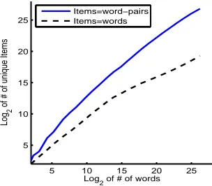
Fig. 1 helps us understand the seriousness of the situation. It plots the number of unique word-s/word pairs versus the total number of words in

5 10 15 20 25

5 10 15 20 25

Log

2 of # of words

Log

2

of # of unique Items

Items=word−pairs Items=words

Figure 1:Token Type Curve

a corpus of size 577MB. Note that the plot is in log-log scale. This78 million word corpus gen-erates63thousand unique words and118million unique word pairs. As expected, the rapid increase in number of unique word pairs is much larger than the increase in number of words. Hence, it shows that it is computationally infeasible to com-pute counts of all word pairs with a giant corpora using conventional main memory of8GB.

Storing only the118million unique word pairs in this corpus require1.9GB of disk space. This space can be saved by avoiding storing the word pair itself. As a trade-off we are willing to tolerate a small amount of error in the frequency of each word pair. In this paper, we explore sketch tech-niques, especially the Count-Min Sketch, which approximates the frequency of a word pair in the corpus without explicitly storing the word pairs themselves. It turns out that, in this technique, both updating (adding a new word pair or increas-ing the frequency of existincreas-ing word pair) and query-ing (findquery-ing the frequency of a given word pair) are very efficient and can be done in constant time1.

Counts stored in the CM Sketch can be used to compute various word-association measures like

1_{depend only on one of the user chosen parameters}

Pointwise Mutual Information (PMI), and Log-Likelihood ratio. These association scores are use-ful for other NLP applications like word sense disambiguation, speech and character recognition, and computing semantic orientation of a word. In our work, we use computing semantic orientation of a word using PMI as a canonical task to show the effectiveness of CM Sketch for computing as-sociation scores.

In our attempt to advocate the Count-Min sketch to store the frequency of keys (words or word pairs) for NLP applications, we perform both intrinsic and extrinsic evaluations. In our intrinsic evaluation, first we show that low-frequent items are more prone to errors. Second, we show that computing approximate PMI scores from these counts can give the same ranking as Exact PMI. However, we need counters linear in size of stream to achieve that. We use these approximate PMI scores in our extrinsic evaluation of computing se-mantic orientation. Here, we show that we do not need counters linear in size of stream to perform as good as Exact PMI. In our experiments, by us-ing only2billion counters (8GB RAM) we get the same accuracy as for exact PMI scores. The num-ber of these counters is up to30times less than the stream size which is a big memory and space gain without any loss of accuracy.

2 Background

2.1 Large Scale NLP problems

Use of large data in the NLP community is not new. A corpus of roughly1.6Terawords was used by Agirre et al. (2009) to compute pairwise sim-ilarities of the words in the test sets using the MapReduce infrastructure on 2,000cores. Pan-tel et al. (2009) computed similarity between500

million terms in the MapReduce framework over a

200billion words in50hours using200quad-core nodes. The inaccessibility of clusters for every one has attracted the NLP community to use stream-ing, randomized, approximate and sampling algo-rithms to handle large amounts of data.

A randomized data structure called Bloom fil-ter was used to construct space efficient language models (Talbot and Osborne, 2007) for Statis-tical Machine Translation (SMT). Recently, the streaming algorithm paradigm has been used to provide memory and space-efficient platform to deal with terabytes of data. For example, We (Goyal et al., 2009) pose language modeling as

a problem of finding frequent items in a stream of data and show its effectiveness in SMT. Subse-quently, (Levenberg and Osborne, 2009) proposed a randomized language model to efficiently deal with unbounded text streams. In (Van Durme and Lall, 2009b), authors extend Talbot Osborne Mor-ris Bloom (TOMB) (Van Durme and Lall, 2009a) Counter to find the highly rankedkPMI response words given a cue word. The idea of TOMB is similar to CM Sketch. TOMB can also be used to store word pairs and further compute PMI scores. However, we advocate CM Sketch as it is a very simple algorithm with strong guarantees and good properties (see Section 3).

2.2 Sketch Techniques

A sketch is a summary data structure that is used to store streaming data in a memory efficient man-ner. These techniques generally work on an input stream, i.e. they process the input in one direc-tion, say from left to right, without going back-wards. The main advantage of these techniques is that they require storage which is significantly smaller than the input stream length. For typical algorithms, the working storage is sublinear inN, i.e. of the order oflogkN, whereN is the input size andkis some constant which is not explicitly chosen by the algorithm but it is an artifact of it.. Sketch based methods use hashing to map items in the streaming data onto a small-space sketch vec-tor that can be easily updated and queried. It turns out that both updating and querying on this sketch vector requires only a constant time per operation. Streaming algorithms were first developed in the early 80s, but gained in popularity in the late 90s as researchers first realized the challenges of dealing with massive data sets. A good survey of the model and core challenges can be found in (Muthukrishnan, 2005). There has been consid-erable work on coming up with different sketch techniques (Charikar et al., 2002; Cormode and Muthukrishnan, 2004; Li and Church, 2007). A survey by (Rusu and Dobra, 2007; Cormode and Hadjieleftheriou, 2008) comprehensively reviews the literature.

3 Count-Min Sketch

on the data stream such as point, range and in-ner product queries to be approximately answered very quickly. It can also be applied to solve the finding frequent items problem (Manku and Mot-wani, 2002) in a data stream. In this paper, we are only interested in point queries. The aim of a point query is to estimate the count of an item in the in-put stream. For other details, the reader is referred to (Cormode and Muthukrishnan, 2004).

Given an input stream of word pairs of lengthN and user chosen parametersδandǫ, the algorithm stores the frequencies of all the word pairs with the following guarantees:

• All reported frequencies are within the true frequencies by at mostǫN with a probability of at leastδ.

• The space used by the algorithm is O(1

ǫlog

1

δ).

• Constant time of O(log(1

δ)) per each update and query operation.

3.1 CM Data Structure

A Count-Min Sketch with parameters (ǫ,δ) is rep-resented by a two-dimensional array with widthw and depthd:



 

sketch[1,1] · · · sketch[1,w] ..

. . .. ... sketch[d,1] · · · sketch[d,w]



 

Among the user chosen parameters,ǫcontrols the amount of tolerable error in the returned count and δcontrols the probability with which the returned count is not within the accepted error. These val-ues ofǫandδdetermine the width and depth of the two-dimensional array respectively. To achieve the guarantees mentioned in the previous section, we setw=2_ǫ andd=log(1

δ). The depthddenotes the number of pairwise-independent hash func-tions employed by the algorithm and there exists an one-to-one correspondence between the rows and the set of hash functions. Each of these hash functionshk:{1. . . N} → {1. . . w}(1≤k≤d) takes an item from the input stream and maps it into a counter indexed by the corresponding hash function. For example,h2(w) = 10indicates that

the word pairwis mapped to the10th_{position in} the second row of the sketch array. Thesedhash functions are chosen uniformly at random from a pairwise-independent family.

Figure 2: Update Procedure for CM sketch and conserva-tive update (CU)

Initially the entire sketch array is initialized with zeros.

Update Procedure: When a new item (w,c) ar-rives, where w is a word pair and cis its count2, one counter in each row, as decided by its corre-sponding hash function, is updated byc. Formally,

∀1≤k≤d

sketch[k,hk(w)]←sketch[k,hk(w)]+c

This process is illustrated in Fig. 2 CM. The item (w,2) arrives and gets mapped to three positions, corresponding to the three hash functions. Their counts before update were (4,2,1) and after update they become (6,4,3). Note that, since we are using a hash to map a word into an index, a collision can occur and multiple word pairs may get mapped to the same counter in any given row. Because of this, the values stored by thedcounters for a given word pair tend to differ.

Query Procedure: The querying involves

find-ing the frequency of a given item in the input stream. Since multiple word pairs can get mapped into same counter and the observation that the counts of items are positive, the frequency stored by each counter is an overestimate of the true count. So in answering the point query, we con-sider all the positions indexed by the hash func-tions for the given word pair and return the mini-mum of all these values. The answer to Query(w) is:

ˆ

c=minksketch[k,hk(w)]

Note that, instead of positive counts if we had neg-ative counts as well then the algorithm returns the median of all the counts and the bounds we dis-cussed in Sec. 3 vary. In Fig. 2 CM, for the word pair wit takes the minimum over (6,4,3) and re-turns3as the count of word pair w.

2

Both update and query procedures involve eval-uatingdhash functions and a linear scan of all the values in those indices and hence both these pro-cedures are linear in the number of hash functions. Hence both these steps requireO(log(1

δ))time. In our experiments (see Section 4.2), we found that a small number of hash functions are sufficient and we use d=3. Hence, the update and query oper-ations take only a constant time. The space used by the algorithm is the size of the array i.e. wd counters, wherewis the width of each row.

3.2 Properties

Apart from the advantages of being space efficient, and having constant update and constant querying time, the Count-Min sketch has also other advan-tages that makes it an attractive choice for NLP applications.

• Linearity: given two sketchess1ands2

com-puted (using the same parametersw andd) over different input streams, the sketch of the combined data stream can be easily ob-tained by adding the individual sketches in O(1_ǫlog1

δ) time which is independent of the stream size.

• The linearity is especially attractive because, it allows the individual sketches to be com-puted independent of each other. Which means that it is easy to implement it in dis-tributed setting, where each machine com-putes the sketch over a sub set of corpus.

• This technique also extends to allow the dele-tion of items. In this case, to answer a point query, we should return the median of all the values instead of the minimum value.

3.3 Conservative Update

Estan and Varghese introduce the idea of conser-vative update (Estan and Varghese, 2002) in the context of networking. This can easily be used with CM Sketch to further improve the estimate of a point query. To update an item, word pair, w with frequency c, we first compute the frequency

ˆ

cof this item from the existing data structure and the counts are updated according to:∀1≤k≤d

sketch[k,hk(w)]←max{sketch[k,hk(w)],ˆc+c}

The intuition is that, since the point query returns the minimum of all thedvalues, we will update

a counter only if it is necessary as indicated by the above equation. Though this is a heuristic, it avoids the unnecessary updates of counter values and thus reduces the error.

The process is also illustrated in Fig. 2CU. When an item “w” with a frequency of 2arrives in the stream, it gets mapped into three positions in the sketch data structure. Their counts before update were (4,2,1) and the frequency of the item is1(the minimum of all the three values). In this particular case, the update rule says that increase the counter value only if its updated value is less than ˆc+ 2 = 3. As a result, the values in these counters after the update become (4,3,3).

However, if the value in any of the counters is already greater than 3 e.g. 4, we cannot at-tempt to correct it by decreasing, as it could con-tain the count for other items hashed at that posi-tion. Therefore, in this case, for the first counter we leave the value 4unchanged. The query pro-cedure remains the same as in the previous case. In our experiments, we found that employing the conservative update reduces the Average Relative Error (ARE) of these counts approximately by a factor of 2. (see Section 4.2). But unfortunately, this update prevents deletions and items with neg-ative updates cannot be processed3.

4 Intrinsic Evaluations

To show the effectiveness of the Count-Min sketch in the context of NLP, we perform intrinsic evalu-ations. The intrinsic evaluations are designed to measure the error in the approximate counts re-turned by CMS compared to their true counts. By keeping the total size of the data structure fixed, we study the error by varying the width and the depth of the data structure to find the best setting of the parameters for textual data sets. We show that using conservative update (CU) further im-proves the quality of counts over CM sketch.

4.1 Corpus Statistics

Gigaword corpus (Graff, 2003) and a copy of web crawled by (Ravichandran et al., 2005) are used to compute counts of words and word pairs. For both the corpora, we split the text into sentences, tokenize and convert into lower-case. We generate words and word pairs (items) over a sliding win-dow of size14. Unlike previous work (Van Durme

Corpus Sub Giga 50% 100%

set word Web Web

Size

.15 6.2 15 31

GB # of sentences

2.03 60.30 342.68 686.63 (Million)

# of words

19.25 858.92 2122.47 4325.03 (Million)

Stream Size

0.25 19.25 18.63 39.05 10 (Billion)

Stream Size _{0.23 25.94 18.79 40.00} 14 (Billion)

Table 1: Corpus Description

and Lall, 2009b) which assumes exact frequen-cies for words, we store frequenfrequen-cies of both the words and word pairs in the CM sketch4_{. Hence,}

the stream size in our case is the total number of words and word pairs in a corpus. Table 1 gives the characteristics of the corpora.

Since, it is not possible to compute exact fre-quencies of all word pairs using conventional main memory of 8GB from a large corpus, we use a subset of2million sentences (Subset) from Giga-word corpus for our intrinsic evaluation. We store the counts of all words and word pairs (occurring in a sliding window of length14) from Subset us-ing the sketch and also the exact counts.

4.2 Comparing CM and CU counts and tradeoff between width and depth

To evaluate the amount of over-estimation in CM and CU counts compared to the true counts, we first group all items (words and word pairs) with same true frequency into a single bucket. We then compute the average relative error in each of these buckets. Since low-frequent items are more prone to errors, making this distinction based on fre-quency lets us understand the regions in which the algorithm is ovestimating. Average Relative er-ror (ARE) is defined as the average of absolute dif-ference between the predicted and the exact value divided by the exact value over all the items in each bucket.

ARE= 1

N N X

i=1

|Exacti−Predictedi| Exacti

Where Exact and Predicted denotes values of exact and CM/CU counts respectively; N denotes the number of items with same counts in a bucket.

In Fig. 3(a), we fixed the number of counters to50million with four bytes of memory per each

4_{Though a minor point, it allows to process more text.}

counter (thus it only requires 200 MB of main memory). Keeping the total number of counters fixed, we try different values of depth (2,3,5and

7) of the sketch array and in each case the width is set to 50_dM. The ARE curves in each case are shown in Fig. 3(a). There are three main observa-tions: First it shows that most of the errors occur on low frequency items. For frequent items, in al-most all the different runs the ARE is close to zero. Secondly, it shows that ARE is significantly lower (by a factor of two) for the runs which use conser-vative update (CUx run) compared to the runs that use direct CM sketch (CMx run). The encouraging observation is that, this holds true for almost all different (width,depth) settings. Thirdly, in our ex-periments, it shows that using depth of3gets com-paratively less ARE compared to other settings.

To be more certain about this behavior with re-spect to different settings of width and depth, we tried another setting by increasing the number of counters to100million. The curves in 3(b) follow a pattern which is similar to the previous setting. Low frequency items are more prone to error com-pared to the frequent ones and employing conser-vative update reduces the ARE by a factor of two. In this setting, depth 3and5do almost the same and get lowest ARE. In both the experiments, set-ting the depth to three did well and thus in the rest of the paper we fix this parameter to three.

Fig. 4 studies the effect of the number of coun-ters in the sketch (the size of the two-dimensional sketch array) on the ARE. Using more number of counters decreases the ARE in the counts. This is intuitive because, as the length of each row in the sketch increases, the probability of collision de-creases and hence the array is more likely to con-tain true counts. By using 200million counters, which is comparable to the length of the stream

230million (Table. 1), we are able to achieve al-most zero ARE over all the counts including the rare ones5_{. Note that the actual space required}

to represent the exact counts is almost two times more than the memory that we use here because there are230million word pairs and on an aver-age each word is eight characters long and requires eight bytes (double the size of an integer). The summary of this Figure is that, if we want to pre-serve the counts of low-frequent items accurately, then we need counters linear in size of stream.

5

Even with other datasets we found that using counters linear in the size of the stream leads to ARE close to zero∀

0 2 4 6 8 10 12 0

0.5 1 1.5 2 2.5 3 3.5 4

Log

2 of true frequency counts of words/word−pairs

Average Relative Error

CM7 CM5 CM3 CM2 CU7 CU5 CU3 CU2

(a) 50M counters

0 2 4 6 8 10 12

0 0.1 0.2 0.3 0.4 0.5 0.6 0.7 0.8

Log₂ of true frequency counts of words/word−pairs

Average Relative Error

CM7 CM5 CM3 CM2 CU7 CU5 CU3 CU2

(b) 100M counters

Figure 3:Comparing50and100million counter models with different (width,depth) settings. The notation CMx represents the Count-Min Sketch with a depth of ’x’ and CUx represents the CM sketch along with conservative update and depth ’x’.

0 2 4 6 8 10 12

0 1 2 3 4 5 6

Log

2 of true frequency counts of words/word−pairs

Average Relative Error

20M 50M 100M 200M

Figure 4:Comparing different size models with depth3

4.3 Evaluating the CU PMI ranking

In this experiment, we compare the word pairs as-sociation rankings obtained using PMI with CU and exact counts. We use two kinds of measures, namely accuracy and Spearman’s correlation, to measure the overlap in the rankings obtained by both these approaches.

4.3.1 PointWise Mutual Information

The Pointwise Mutual Information (PMI) (Church and Hanks, 1989) between two wordsw1andw2

is defined as:

P M I(w1, w2) = log2

P(w1, w2)

P(w1)P(w2)

Here,P(w1, w2)is the likelihood thatw1andw2

occur together, andP(w1)andP(w2)are their

in-dependent likelihoods respectively. The ratio be-tween these probabilities measures the degree of statistical dependence betweenw1andw2.

4.3.2 Description of the metrics

Accuracy is defined as fraction of word pairs that are found in both rankings to the size of top ranked word pairs.

Accuracy=|CP-WPs∩EP-WPs| |EP-WPs|

Where CP-WPs represent the set of top rankedK word pairs under the counts stored using the CU sketch and EP-WPs represent the set of top ranked word pairs with the exact counts.

Spearman’s rank correlation coefficient (ρ) computes the correlation between the ranks of each observation (i.e. word pairs) on two variables (that are top N CU-PMI and exact-PMI values). This measure captures how different the CU-PMI ranking is from the Exact-PMI ranking.

ρ= 1− 6

P d2

i F(F2₋₁₎

Wherediis the difference between the ranks of a word pair in both rankings andF is the number of items found in both sets.

Intuitively, accuracy captures the number of word pairs that are found in both the sets and then Spearman’s correlation captures if the relative or-der of these common items is preserved in both the rankings. In our experimental setup, both these measures are complimentary to each other and measure different aspects. If the rankings match exactly, then we get an accuracy of 100% and a correlation of1.

4.3.3 Comparing CU PMI ranking

Counters 50M 100M 200M

TopK Acc ρ Acc ρ Acc ρ

50 .20 -0.13 .68 .95 .92 1.00 100 .18 .31 .77 .80 .96 .95 200 .21 .68 .73 .86 .97 .99 500 .24 .31 .71 .97 .95 .99 1000 .33 .17 .74 .87 .95 .98 5000 .49 .38 .82 .82 .96 .97

Table 2: Evaluating the PMI rankings obtained using CM Sketch with conservative update (CU) and Exact counts

in size of stream (230M) results in better rank-ing (i.e. close to the exact rankrank-ing). For example, with200Mcounters, among the top50word pairs produced using the CU counts, we found46pairs in the set returned by using exact counts. Theρ score on those word pairs is1means that the rank-ing of these46items is exactly the same on both CU and exact counts. We see the same phenom-ena for200M counters with other TopKvalues. While both accuracy and the ranking are decent with100M counters, if we reduce the number of counters to say50M, the performance degrades.

Since, we are not throwing away any infrequent items, PMI will rank pairs with low frequency counts higher (Church and Hanks, 1989). Hence, we are evaluating the PMI values for rare word pairs and we need counters linear in size of stream to get almost perfect ranking. Also, using coun-ters equal to half the length of the stream is decent. However, in some NLP problems, we are not inter-ested in low-frequency items. In such cases, even using space less than linear in number of coun-ters would suffice. In our extrinsic evaluations, we show that using space less than the length of the stream does not degrades the performance.

5 Extrinsic Evaluations

5.1 Experimental Setup

To evaluate the effectiveness of CU-PMI word association scores, we infer semantic orientation (S0) of a word from CU-PMI and Exact-PMI scores. Given a word, the task of finding the SO (Turney and Littman, 2002) of the word is to iden-tify if the word is more likely to be used in positive or negative sense. We use a similar framework as used by the authors6to infer the SO. We take the seven positive words (good, nice, excellent, posi-tive, fortunate, correct, and superior) and the nega-tive words (bad, nasty, poor, neganega-tive, unfortunate,

6

We compute this score slightly differently. However, our main focus is to show that CU-PMI scores are useful.

wrong, and inferior) used in (Turney and Littman, 2002) work. The SO of a given word is calculated based on the strength of its association with the seven positive words, and the strength of its asso-ciation with the seven negative words. We com-pute the SO of a word ”w” as follows:

SO-PMI(W) = P M I(+, w)−P M I(−, w)

PMI(+,W) = X

p∈P words

log hits(p, w)

hits(p)·hits(w)

PMI(-,W) = X

n∈N words

log hits(n, w)

hits(n)·hits(w)

Where, Pwords and Nwords denote the seven pos-itive and negative prototype words respectively.

We compute SO score from different sized cor-pora (Section 4.1). We use the General Inquirer lexicon7 (Stone et al., 1966) as a benchmark to evaluate the semantic orientation scores similar to (Turney and Littman, 2002) work. Words with multiple senses have multiple entries in the lexi-con, we merge these entries for our experiment. Our test set consists of 1619 positive and 1989

negative words. Accuracy is used as an evaluation metric and is defined as the fraction of number of correctly identified SO words.

Accuracy= Correctly Identified SO Words∗100

Total SO words

5.2 Results

We evaluate SO of words on three different sized corpora: Gigaword (GW) 6.2GB, GigaWord +

50% of web data (GW+WB1) 21.2GB and Gi-gaWord + 100% of web data (GW+WB2)31GB. Note that computing the exact counts of all word pairs on these corpora is not possible using main memory, so we consider only those pairs in which one word appears in the prototype list and the other word appears in the test set.

We compute the exact PMI (denoted using Ex-act) scores for pairs of test-set wordsw1and

proto-type wordsw2using the above data-sets. To

com-pute PMI, we count the number of hits of individ-ual wordsw1andw2and the pair (w1,w2) within a

sliding window of sizes10and14over these data-sets. After computing the PMI scores, we compute SO score for a word using SO-PMI equation from Section 5.1. If this score is positive, we predict the word as positive. Otherwise, we predict it as

7

Model Accuracy window 10 Accuracy window 14

#of counters Mem. Usage GW GW+WB1 GW+WB2 GW GW+WB1 GW+WB2 Exact n/a 64.77 75.67 77.11 64.86 74.25 75.30

500M 2GB 62.98 71.09 72.31 63.21 69.21 70.35 1B 4GB 62.95 73.93 75.03 63.95 72.42 72.73

2B 8GB 64.69 75.86 76.96 65.28 73.94 74.96

Table 3:Evaluating Semantic Orientation of words with different # of counters of CU sketch with increasing amount of data on window size of 10 and 14. Scores are evaluated using Accuracy metric.

negative. The results on inferring correct SO for a word w with exact PMI (Exact) are summarized in Table 3. It (the second row) shows that increas-ing the amount of data improves the accuracy of identifying the SO of a word with both the win-dow sizes. The gain is more prominent when we add50% of web data in addition to Gigaword as we get an increase of more than10% in accuracy. However, when we add the remaining50% of web data, we only see an slight increase of1% in accu-racy8. Using words within a window of10gives better accuracy than window of14.

Now, we use our CU Sketches of500 million (500M),1billion (1B) and2billion (2B) coun-ters to compute CU-PMI. These sketches contain the number of hits of all words/word pairs (not just the pairs of test-set and prototype words) within a window size of 10 and 14 over the whole data-set. The results in Table 3 show that even with CU-PMI scores, the accuracy improves by adding more data. Again we see a significant increase in accuracy by adding50% of web data to Gigaword over both window sizes. The increase in accuracy by adding the rest of the web data is only1%.

By using 500M counters, accuracy with CU-PMI are around4% worse than the Exact. How-ever, increasing the size to 1B results in only 2

% worse accuracy compared to the Exact. Go-ing to2Bcounters (8GB of RAM), results in ac-curacy almost identical to the Exact. These re-sults hold almost the same for all the data-sets and for both the window sizes. The increase in accuracy comes at expense of more memory Us-age. However,8GB main memory is not large as most of the conventional desktop machines have this much RAM. The number of 2B counters is less than the length of stream for all the data-sets. For GW, GW+WB1 and GW+WB2,2Bcounters are 10, 20and 30times smaller than the stream size. This shows that using counters less than the stream length does not degrade the performance.

8

These results are similar to the results reported in (Tur-ney and Littman, 2002) work.

The advantage of using Sketch is that it con-tains counts for all words and word pairs. Suppose we are given a new word to label it as positive or negative. We can find its exact PMI in two ways: First, we can go over the whole corpus and com-pute counts of this word with positive and nega-tive prototype words. This procedure will return PMI in time needed to traverse the whole corpus. If the corpus is huge, this could be too slow. Sec-ond option is to consider storing counts of all word pairs but this is not feasible as their number in-creases rapidly with increase in data (see Fig. 1). Therefore, using a CM sketch is a very good al-ternative which returns the PMI in constant time by using only8GB of memory. Additionally, this Sketch can easily be used for other NLP applica-tions where we need word-association scores.

6 Conclusion

We have explored the idea of the CM Sketch, which approximates the frequency of a word pair in the corpus without explicitly storing the word pairs themselves. We used the idea of a conserva-tive update with the CM Sketch to reduce the av-erage relative error of its approximate counts by a factor of 2. It is an efficient, small-footprint method that scales to at least 37GB of web data in just2billion counters (8GB main memory). In our extrinsic evaluations, we found that CU Sketch is as effective as exact PMI scores.

Word-association scores from CU Sketch can be used for other NLP tasks like word sense disam-biguation, speech and character recognition. The counts stored in CU Sketch can be used to con-struct small-space randomized language models. In general, this sketch can be used for any applica-tion where we want to query a count of an item.

Acknowledgments

References

Eneko Agirre, Enrique Alfonseca, Keith Hall, Jana Kravalova, Marius Pas¸ca, and Aitor Soroa. 2009. A study on similarity and relatedness using distri-butional and wordnet-based approaches. In NAACL

’09: Proceedings of Human Language Technolo-gies: The 2009 Annual Conference of the North American Chapter of the Association for Computa-tional Linguistics.

Thorsten Brants, Ashok C. Popat, Peng Xu, Franz J.

Och, and Jeffrey Dean. 2007. Large language

models in machine translation. In Proceedings of

the 2007 Joint Conference on Empirical Methods in Natural Language Processing and Computational Natural Language Learning (EMNLP-CoNLL).

Moses Charikar, Kevin Chen, and Martin

Farach-colton. 2002. Finding frequent items in data

streams.

K. Church and P. Hanks. 1989. Word Association Norms, Mutual Information and Lexicography. In

Proceedings of the 27th Annual Meeting of the Asso-ciation for Computational Linguistics, pages 76–83,

Vancouver, Canada, June.

Graham Cormode and Marios Hadjieleftheriou. 2008. Finding frequent items in data streams. In VLDB.

Graham Cormode and S. Muthukrishnan. 2004. An improved data stream summary: The count-min sketch and its applications. J. Algorithms.

Cristian Estan and George Varghese. 2002. New direc-tions in traffic measurement and accounting.

SIG-COMM Comput. Commun. Rev., 32(4).

Amit Goyal, Hal Daum´e III, and Suresh Venkatasub-ramanian. 2009. Streaming for large scale NLP:

Language modeling. In North American

Chap-ter of the Association for Computational Linguistics (NAACL).

D. Graff. 2003. English Gigaword. Linguistic Data Consortium, Philadelphia, PA, January.

Abby Levenberg and Miles Osborne. 2009.

Stream-based randomised language models for SMT. In

Proceedings of the 2009 Conference on Empirical Methods in Natural Language Processing, pages

756–764, Singapore, August. Association for Com-putational Linguistics.

Ping Li and Kenneth W. Church. 2007. A sketch algo-rithm for estimating two-way and multi-way associ-ations. Comput. Linguist., 33(3).

G. S. Manku and R. Motwani. 2002. Approximate frequency counts over data streams. In Proceedings

of the 28th International Conference on Very Large Data Bases.

S. Muthukrishnan. 2005. Data streams: Algorithms and applications. Foundations and Trends in

Theo-retical Computer Science, 1(2).

Patrick Pantel, Eric Crestan, Arkady Borkovsky,

Ana-Maria Popescu, and Vishnu Vyas. 2009.

Web-scale distributional similarity and entity set

expan-sion. In Proceedings of the 2009 Conference on

Empirical Methods in Natural Language Process-ing, pages 938–947, Singapore, August. Association

for Computational Linguistics.

S. Patwardhan and E. Riloff. 2006. Learning Domain-Specific Information Extraction Patterns from the Web. In Proceedings of the ACL 2006 Workshop on

Information Extraction Beyond the Document.

Deepak Ravichandran, Patrick Pantel, and Eduard Hovy. 2005. Randomized algorithms and nlp: using locality sensitive hash function for high speed noun clustering. In ACL ’05: Proceedings of the 43rd

An-nual Meeting on Association for Computational Lin-guistics.

Florin Rusu and Alin Dobra. 2007. Statistical analysis of sketch estimators. In SIGMOD ’07. ACM.

Philip J. Stone, Dexter C. Dunphy, Marshall S. Smith,

and Daniel M. Ogilvie. 1966. The General

In-quirer: A Computer Approach to Content Analysis.

MIT Press.

David Talbot and Miles Osborne. 2007. Smoothed Bloom filter language models: Tera-scale LMs on the cheap. In Proceedings of the 2007 Joint

Con-ference on Empirical Methods in Natural Language Processing and Computational Natural Language Learning (EM NLP-CoNLL).

Peter D. Turney and Michael L. Littman. 2002.

Unsupervised learning of semantic orientation

from a hundred-billion-word corpus. CoRR,

cs.LG/0212012.

Peter D. Turney. 2008. A uniform approach to analo-gies, synonyms, antonyms, and associations. In

Pro-ceedings of COLING 2008.

Benjamin Van Durme and Ashwin Lall. 2009a. Prob-abilistic counting with randomized storage. In

IJ-CAI’09: Proceedings of the 21st international jont conference on Artifical intelligence, pages 1574–

1579.

Benjamin Van Durme and Ashwin Lall. 2009b.

Streaming pointwise mutual information. In