Principal Components Analysis with Spline
Optimal Transformations for Continuous Data
Nuno Lavado,
Member, IAENG,
and Teresa Calapez
Abstract—A new approach to generalize Principal Compo-nents Analysis in order to handle nonlinear structures has been recently proposed by the authors: quasi-linear PCA (qlPCA). It includes spline transformation of the original variables and the qualifier quasi was chosen to emphasize the exclusive use of linear splines. Alternating least squares fitting of a suitable objective loss function is the mechanism for achieving spline optimal transformation and nonlinear principal components. Optimal transformations are explicitly known after convergence and allow a straightforward projection of new observations onto the nonlinear principal components space as well as reconstruction the original variables. QlPCA reports model summary in a linear PCA fashion and allows the introduction of the piecewise loadingsconcept. This paper provides further details on qlPCA and its properties. Results of a simulation study are also presented.
Index Terms—nonlinear principal components analysis, qlPCA, linear PCA, CATPCA.
I. INTRODUCTION
P
RINCIPAL Components Analysis (PCA) being probably the most common descriptive multivariate technique for seeking linear structure in data, it is unsurprising to find a number of attempts at generalizing it in order to handle nonlinear structures. The concept behind PCA is to project the original data, which includes noise and redundant variables, into a latent space with the objective of capturing its true dimensionality.All descriptive methods for dimension reduction share the same basic premise and general objectives: the original data can be viewed as a collection of n points in some high m-dimensional space, the points corresponding to sample individuals and the dimensions to measured variables, and we seek for a suitable lowp-dimensional approximation in which the points are positioned such that as much information as possible is retained from the original space. By reducing the dimensionality, one can interpret few components rather than a large number of variables. Different interpretations of the phrase “as much information as possible” lead to the different multivariate techniques for dimension reduction.
One technique can be described aslinearwhen the high-dimensional set of coordinates is replaced by another in a one-to-onelinearrelation with it. All attempts to generalize PCA in order to handle nonlinear structures, the gener-ally denominated Nonlinear Principal Components Analysis (NLPCA), share the basic premise and general objectives
Submitted October 27, 2011.
N. Lavado is with the Department of Physics and Mathematics, Coimbra Institute of Engineering (ISEC), Coimbra, Portugal and with the research unit Instituto Universit´ario de Lisboa (ISCTE-IUL), Unidade de Investigac¸˜ao em Desenvolvimento Empresarial (Unide-IUL), Lisboa, Portugal, e-mail: [email protected].
T. Calapez is with the research unit Instituto Universit´ario de Lisboa (ISCTE-IUL), Unidade de Investigac¸˜ao em Desenvolvimento Empresarial (Unide-IUL), Lisboa, Portugal, e-mail: [email protected].
mentioned, but they address the nonlinearity problem by relaxing the linear restrictions between spaces.
An early attempt to generalize PCA was made by Gnanadesikan and Wilk in the ‘60’s. The idea was to extend the m-dimensional space by adding nonlinear functions of the original variables (quadratic and higher order terms) and then perform PCA on the expanded set of variables [1]. The key to this approach was to decide on the appropriate dimensionality of the extended space as well as the non-linear relationships between the original variables needed to describe the system. This drawback was removed in the ‘90’s by Sch¨olkopf [2] using a function from the original m-dimensional space onto an arbitrarily high-dimensional space (known as feature space in the machine learning community) which “automatically” carries out the nonlinear mapping. It turns out that this mapping can be performed implicitly by using kernel functions and therefore does not need to be specified. This approach, known as kernel PCA, applies linear PCA on the feature space. Recently, Kruger [3] reviews existing work on NLPCA and points out that it can be divided into the utilization of autoassociative neural networks, principal curves and manifolds, kernel approaches or the combination of these approaches.
NLPCA’s most known approaches among researchers deal-ing with continuous variables do not include the state-of-the-art to perform NLPCA for ordinal and nominal data, CATegorical PCA (CATPCA). We refer to a continuous variable as one with small marginal frequencies on every value, typically one or two. CATPCA performs quite well when applied to categorical variables and is more appropriate when [4]: (1) the data at hand contains categorical variables, and/or (2) the variables in the data are (or may be) nonlin-early related to each other. If the variables are nonlinnonlin-early related, CATPCA will be able to account for more of the variance in the data, and may enhance the interpretation of the solution compared to linear PCA. CATPCA’s algorithm was developed in the ‘90’s as an algorithm for categorical data analysis, thus for dealing with integer valued variables. Continuous data need to undergo a discretization process before the algorithm starts. Various discretization options are available for recoding continuous data within the procedure and one can always recode data beforehand. Our proposal is to adjust the algorithm to allow continuous values directly so that researchers dealing with continuous variables avoid thinking that some information is being neglect.
A new approach on generalizing PCA in order to handle nonlinear structures have been recently proposed by the au-thors [5], quasi-linear PCA (qlPCA). The proposed approach was inspired by the Gifi system [6], also called Homogeneity Analysis, in particular by its natural successor CATPCA. QlPCA recovers the spline based algorithm in CATPCA, and introduces continuous variables into the framework directly
IAENG International Journal of Applied Mathematics, 41:4, IJAM_41_4_14
without the need of any discretization process. Thus, this approach is more precise with regard to continuous variables and provides a better approximation of a strictly nonlinear analysis, becoming a valid option to perform NLPCA for those variables.
This paper provides further details on qlPCA and its properties. A brief review on splines is provided in the next section followed by an overview of the Gifi system and CATPCA in section III. A suitable objective (loss) function is defined in section IV as well as details on qlPCA’s algorithm. The main properties of qlPCA are reported in section V: model summary, choosing the appropriate num-ber of components, projecting new observations onto the nonlinear principal components’ space, reconstruction and
piecewise loadings’ definition. Results of a simulation study are provided on section VI.
II. SPLINE’S BRIEF REVIEW
Low order polynomial spline functions play an important roll in our quasi-linear PCA (qlPCA) proposal. In this section it will be provided the main results on spline functions that will be useful for our purposes. For a comprehensive overview see [7], [8].
A functionf over [a, b], is apolynomial spline of degree v if within any subinterval is defined by a polynomial of degreev that join smoothly with adjacent ones. Although it is possible to define several degrees of smoothness at the boundaries of each subinterval [9], in the most common situations adjacent polynomials have matching derivatives up to orderv−1at each boundary point in the interior of[a, b]. Examples:
1) The first order (or zero degree) spline is a piecewise constant function, discontinuous at the interior knots; 2) The second order spline is a continuous piecewise
linear function;
3) The third order spline is a piecewise quadratic function with matching first derivatives at the interior knots.
It can be shown [7], [8] that the set of splines of degree v with r interior knots is a linear space of functions, with dimensionw=v+ 1 +r, equal to the spline’s order plus the number of interior knots. In 1966, Curry and Schoenberg [7] have built a basis, what they calledB-splines, which revealed to be especially convenient for computation.
In order to provide a spline’s representation convenient from the points of view of application and computation, smoothness conditions are incorporated into a knot sequence {t}={t1, . . . , t2v+r+2} where:
1) t1≤. . .≤t2v+r+2;
2) t1=. . .=tv+1=a;
3) tv+r+2=. . .=t2v+r+2=b;
4) tv+2, . . . , tv+r+1 are ther interior knots.
Given the knot sequence{t}, spline’s basis of orderv+ 1
is defined, for allq= 1,2, . . . , w, by the recursive relation
Bq[1](x) = {
1 , tq ≤x < tq+1
0 , otherwise ,
B[qv+1](x) = x−tq
tq+v−tq
Bq[v](x) + tq+v+1−x
tq+v+1−tq+1
Bq[v+1] (x),
where x−tq
tq+v−tq
Bq[v](x) and tq+v+1−x tq+v+1−tq+1
Bq[v+1] (x)
are equal to zero when the denominators are zero.
Another set of basis splines particularly appealing to statisticians is theM-spline basis,
Mq[v+1]= v+ 1
tq+v+1−tq
Bq[v+1] , q= 1, . . . , w. (1) It can be shown [8] that Mq[v+1] is positive and less
than 1 over ]tq, tq+v+1[, zero elsewhere and also that
∫ ∞
−∞
Mq[v+1](x)dx= 1. ThusMq[v+1] is a probability
den-sity function. Monotone transformations can be obtained using a monotone splines’ basis together with nonnegative coefficients. Since eachM-splinehas the properties of a prob-ability density function, another basis can be obtained using the corresponding distribution function: integrated splines or
I-splines[10].
Given the knot sequence{t}theI-spline of orderv+ 2is defined, for allq= 1,2, . . . , w by
Iq[v+2](x) = ∫ x
−∞
Mq[v+1](u)du. (2)
Since eachM-spline is a piecewise polynomial of degree v, the associatedI-splineis a piecewise polynomial of degree v+ 1. Thus, the related space has dimension w+ 1, being w the associated M-spline’s dimensionality. However, by construction, there are only w independent I-splines, thus we can only get the subspace spanned by those. From now on w refers to this subspace’s dimension being w=v+r for a degreev spline withrinterior knots.
From definition it follows thatIq[v+2]is non-constant over ]tq, tq+v+1[, zero bellowtq and one abovetq+v+1.I-splines’
definition by a recurrence relation provides a convenient computational approach. As an illustrative example on how to write aI-splineon a given basis let’s consider linear splines with one interior knot at the median and an input continuous variablexwith minimumm1, medianm2and maximumm3.
The basis elements are the following:
I1(x) =
0, x < m1
x−m1
m2−m1, m1≤x < m2
1 x≥m2
I2(x) =
0, x < m2
x−m2
m3−m2, m2≤x < m3
1 x≥m3
To obtain a spline function of degree one with one interior knot by recurrence it will be necessary in the first place to compute the set of two M-splinesbasis functions of degree zero with one interior knot. As these basis functions are piecewise polynomial of degree zero, each Ii will be a
piecewise polynomial of degree one as needed. Therefore this set ofI-splines basis functions will have two elements. As the entire space of degree one spline functions with one
IAENG International Journal of Applied Mathematics, 41:4, IJAM_41_4_14
interior knot is three-dimensional, the referred set can only generate one of its subspaces.
Figure 1 displays the family of I-splines of degree one defined on[0,1]with one interior knot at the median. Each I-splineis piecewise linear and non-constant over one interval. It also displays an example of the images obtained by each of the three functions (two basis functions and one spline) for a value ofxabove the median (x= 0.58,I1(0.58) = 1,
I2(0.58) = 0.29andf(0.58) = 1.37).
min median 0.58 max
0 0.2 0.4 0.6 0.8 1 1.2 1.4 1.6 1.8 2
original variable
transformed variable
I1 →
I2 → f(h)=1.2I
1+0.6I2→
Fig. 1. Splineof degree one with one interior knot at the median.I1 and I2 are the basis spline functions. Stars represent the images ofxthrough
thesplineobtained as a linear combination ofI1 andI2 with coefficients
1.2 and 0.6, respectively.
A degree n polynomial is determined by n+ 1 points. Therefore, each spline’s segment in Figure 1 can be defined using the points associated with the minimum/median and median/maximum. However, qlPCA algorithm will search for the optimal (as defined in section IV) linear combination ofI-splinesby means of a multivariate linear regression with I1andI2as predictor variables and thus involving whole data
and not only those two points.
III. GIFI SYSTEM ANDCATPCA
For a comprehensive overview on the Gifi system see [6], a recent review is given by [11] and [4].
The central idea of the Gifi system is the notion ofoptimal scaling and its implementation through an alternating least squares (ALS) algorithm. The optimal scaling process as defined by the Gifi system is a transformation of variables by assigning quantitative values to qualitative variables in order to optimize a fixed criterion. Optimality is a relative notion, however, because it is always obtained with respect to the particular data set being analyzed and also depends on the class of admissible transformations. This process (optimal quantification, optimal scaling, optimal scoring) allows non-linear transformations of variables. Variable transformation has become an important tool in data analysis over the last decades. For an historical overview see [4].
One of the optimal scaling procedures for dimension reduction and its SPSS implementation - CATPCA - was de-veloped by the Data Theory Scaling System Group (DTSS), consisting of members of the departments of Education and Psychology of the Faculty of Social and Behavioral Sciences at Leiden University.
The CATPCA algorithm is the state-of-the-art to perform nonlinear PCA for ordinal and nominal data [4] and is
available since 1999 within SPSS Categories 10.0 onwards [12]. The traditional crisp coding of the categorical variables was maintained and the least squares estimation of thespline
coefficients is performed by a multivariate regression on each iteration of the ALS procedure. This approach performs quite well when applied to categorical variables, but it needs an a priori discretization process for quantitative variables or categorical not coded in the traditional way. And by so it is no longer precise with regard to quantitative variables.
CATPCA procedure simultaneously quantifies m categor-ical variables while reducing the dimensionality of the data. The technique consists of finding object scores Xof order n×p (i.e. n = number of cases-objects, p = number of dimensions) and sets of multiple category quantificationsYj
of order kj ×p (i.e. kj = number of categories of each
variable andj= 1, . . . , m) so that the loss function:
σ(X,Y) =n−1∑
j
tr
[
(X−GjYj) ′
(X−GjYj) ]
(3)
is minimal, under the normalization restriction X′X=nI, where:
• Gj is an indicator matrix for variablej, of ordern×kj,
whose elements are 0 when thei-thobject is not in the
r-th category of variable j and 1 when the i-th object is in ther-th category of variablej;
• Iis thep×pidentity matrix.
The algorithm uses ALS to minimize the loss function. It consists of two phases, a model estimation phase and an optimal scaling phase, iteratively alternated until convergence is reached. Both object scores and category quantifications are alternately updated until the optimum is found.
IV. QUASI-LINEARPCA
CATPCA’s algorithm was developed in the ‘90’s as an algorithm for categorical data analysis, thus for dealing with integer valued variables. Continuous data need to undergo a discretization process before the alternating least squares (ALS) algorithm starts. Various discretization options are available for recoding continuous data within the procedure and one can always recode data beforehand. Our proposal is to adjust the algorithm to allow continuous values directly so that researchers dealing with continuous variables avoid thinking that some information is being neglect.
The obvious advantages of incorporating continuous vari-ables directly are:
• the user does not need to care about any discretization process;
• the relative distances within each variables’ values are respected from the start without discretization losses of information.
Although defined and implemented for any given spline’s order and number of interior knots, quasi-linear PCA (qlPCA) refers to linear splines. This approach allows mod-eling several degrees of nonlinear relationships between variables by increasing the number of knots while maintain-ing the transformations stepwise linear. Usmaintain-ing this kind of splines, relative distances are not going to be lost during the optimization process being proportional after convergence
IAENG International Journal of Applied Mathematics, 41:4, IJAM_41_4_14
within any two consecutive interior knots. The main advan-tages of this approach are related to explicitly defining the nonlinear optimal transformation and to identify piecewise loadings (section V).
A. Optimal scaling revisited
LetHben×mstandardized data matrix,pthe number of retained principal components andfj =fj(hj)be the image
vector of hj under the function fj,j = 1, . . . , m. The loss
funtion (3) can be re-written in a more general format into the loss functionσ: Mn×p×Mpm×n→IR so that
σ(X,F) =n−1∑
j
tr
[
(X−Fj(hj)) ′
(X−Fj(hj)) ]
,
(4) with normalization restrictionX′X=nIwhere:
• Fj =
[
fj1 . . . fjp ]
is then×pmatrix collecting the p(different) images of the (same) vector hj; • fjtis the transformed variablejassociated with
dimen-siont,t= 1, . . . , p;
• F=[ F1 . . . Fm ]′
is annm×pmatrix.
Notice that the matrix Fj contains the images of the
same vectorhj, subject topdifferent transformations. If no
restrictions are imposed upon the matrixFj, then each value
of the jth variable receives p different quantifications, one for each retained dimension, in what is commonly called
Multiple quantification[6], [12], [13].
Usually, for continuous variables, order and distance re-strictions are required, which can be imposed by the splines’ parameters (degree, number of interior knots and its place-ment). A familiar way to implement those restrictions starts by imposing rank one restrictions on the matrixFj, on what
is usually calledSingle quantification[6], [12], [13]. Details on Single quantification implementation in the proposed algorithm are given in the next section.
Having fixed the class of admissible transformations for each variable, the purpose is to find the object scores and the transformations that minimize the loss function (4). The main differences between the existing algorithms to solve the loss minimization problem are within the class of admissible transformations. In what splines are concerned, each class of transformations depends on the number of knots, spline’s degree and knots placement. However, while the fitting problem is linear in the basis coefficients, it is highly nonlinear in the knots, and therefore it is desirable to avoid much optimization with respect to them [10]. The choice of a particular spline could be targeted according to the percentage of explained variance (section V.A), by trying different sets of parameters. However, like in all statistical models, nonlinear PCA via splines is susceptible to overfitting when there are too many parameters in the model. In order to prevent overfitting a reasonable amount of data should be in the vicinity of any interior knot [10].
Letfj be the image vector ofhj under a spline of degree
v withrinterior knots, spanned byw=v+r I-splines
fj= w ∑
i=1
αjiI
[v]
ji (hj) =
w ∑
i=1
αjiI
[v]
ji =G△j yj, (5)
where:G△j is the pseudo-indicator matrix for variablej, of order n×w whose columns are the image vectors of the variable j by each of the I-splines basis functions; yj is a
vector of lengthwwhose elements are the linear combination coefficientsyj= [α1α2. . . αw]
′
.
In the previous section the optimal scaling or optimal quantification process was defined within categorical analysis as the transformation of variables by assigning quantitative values to qualitative variables in order to optimize equation (3). Using equation (5) it is possible to re-define the optimal quantification process as a ALS phase that, given the object scores, optimize the vectorsyj in order to minimize the loss
function, or analogously, as the ALS phase that seeks to find the optimal linear combination for each basis spline, given the object scores from the model estimation phase, therefore obtaining the optimal spline transformation to each variable. Notice that if the chosen class of admissible transforma-tions are splines of degree one without interior knots the ALS optimization of equation (4) yields the traditional (linear) PCA solution.
B. QlPCA Algorithm Outline
LetH be n×m standardized data matrix, pthe number of retained principal components, r the number of interior knots andv the spline’s degree.
The qlPCA algorithm uses ALS to minimize (4) using rank one matrices Fj. It consists of two phases iteratively
alter-nated until convergence is reached, an optimal quantification phase and a estimation of object scores phase.
Let H, p, r and v be the algorithm’s inputs. The initial configuration is set as follows.
I. Initialization
1: Zn×p←linearP CA(H)
2: [K,Λ1/2, W]←svd(Z) 3: X←√nKW′
4: aj← 1
nX
′
hj, j= 1, . . . , m
5: [G△1 . . .Gm△]←createIspline(H, v+ 1, r)
Initialization starts by performing a linear PCA on H
retainingpprincipal components on the object scores matrix
Z. This matrix is then orthonormalized (steps 2 and 3, being svda singular value decomposition) such that X′X =nI. On step 4, aj = [a1j. . . asj. . . apj]
′
for each j, being asj the Pearson correlation between variablej and the sth
principal component, also known as component loading. Step 5 computes then×mwmatrix G△= [G△1 . . .G△m]by the iterative procedure described in section II.
II. Alternating Least Squares: optimal quantification phase
(loop across variablesj):
1: y˜j ←Xaj
2: yj ← 1
n((G
△
j )
′
G△j )−1(G△j )′y˜j 3: fj =fj(hj)←G△j yj
4: fj ←fj−fju
IAENG International Journal of Applied Mathematics, 41:4, IJAM_41_4_14
5: fj←
√ n fj
∥fj∥
6: aj← 1
nX
′
fj
Optimal quantification phase updates each variables’ quan-tificationfj (steps 1 to 5) and the vectorsaj (step 6). Least
squares estimation is being used in order to minimize the sum of the squares of the residuals between Xaj and the
transformed variable j (step 2). Notice that step 2 performs a multivariate linear regression with Xaj as the dependent
variable and the columns ofG△j as predictors. This updates
yj, a vector whose elements are the linear combination
coefficients for theI-splines’ basis, which in turn will update each variables’ quantification fj. Each transformed variable
is mean centered (step 4) and normalized to√n(step 5) so that its variance will be one. On step 6,aj is updated, being
now asj, the Pearson correlation between the transformed
variable j and the sth nonlinear principal component, from now on called nonlinear component loading.
III. Alternating Least Squares: estimation of object scores phase
1: Z←∑
j
Fj whereFj =fja ′ j
2: [K,Λ1/2,W]←svd(Z) 3: X←√nKW′
The estimation of object scores phase updates X. Rank one restrictions (Single quantification) are imposed on the n×pmatrix Fj by definingFj =fja
′
j = [fja1j. . .fjapj],
therefore each column of Fj being collinear to fj. In its
general format the loss function (4) used thenm×pmatrix
Fto store multiple quantifications for each variable. This al-gorithm, usingsingle quantificationon every variable allows a re-definition ofFto an×mmatrix whereF= [f1. . .fm].
Thus, by the previous definition, F is the transformed data matrix. Step 1 assigns to Zthe sum ofFj overj (thusZis
a centered matrix). Matrix Zis then orthonormalized (steps 2 and 3) such that X′X=nI; thus object scores will have unitary variance.
IV. Convergence test
The convergence test is performed by testing the difference between two successive values of the loss function (4) against
0.1×10⁻⁵. The algorithm goes back to II if convergence is not reached or stops if the maximum number of iterations is reached.
After convergence, qlPCA will produce the following outputs:
• X-n×pmatrix containing the nonlinear objects scores;
• F-n×mmatrix containing the optimally transformed variables;
• A= [a1. . .am]-p×mmatrix with nonlinear loadings; • y-mw-vector with optimal coefficients associated with
m I-splinesbasis.
C. Some notes on the computer program
QlPCA algorithm has been implemented through (freely downloadable) MATLAB m-files. MATLAB version 2009b was used and a MATLAB GUI (Graphical User Interface) and can be obtained from the correspondent author.
The computer program is in a preliminary form since at the moment it only allows the same type of splines for all variables.
For the computation of the I-splines basis we have de-signed our own program based on the theoretical foundations in [7], [8] and [10]. At the moment nothing in our algorithm ensures that a nondecreasing spline is obtained. However the basis coefficients are computed so that they minimize the loss function. Therefore, if a nondecreasing spline is the optimal transformation for the existing structure, it will emerge naturally. This will be exemplified in section VI.
Applying qlPCA involves trying out different options regarding spline’s order and the number of interior knots. Linear splines have several advantages (see next section) but the user can always try higher order splines. The actual implementation does not allow users to choose specific locations for knots: they are always placed at equally spaced percentiles and thus each interval contains approximately the same number of data points. It was already mentioned that in order to prevent overfitting a reasonable amount of data should be in the vicinity of any interior knot [10]. The cause of overfitting is related to step II.2 of qlPCA’s algorithm, where a multivariate regression with w = v+r (spline’s degree plus the number of interior knots) predictor variables is performed. With our knots placement option, preventing overfitting is a matter of the number of available individuals, n, versusw. There is no consensus in the literature regarding the minimum number of available observations per predictor on linear multivariate regression, but a value of 10 to 15 ob-servations per predictor is commonly referred. Whatever the rule of thumb chosen, its adaption to the qlPCA framework implies multiplying that number byw.
V. PROPERTIES OF QUASI LINEARPCA
The qlPCA algorithm will take advantage of low order splines, without limitation concerning the number of interior knots, in order to achieve nonlinear PCA as a straightforward generalization of the traditional PCA including its measures of performance and interpretation. In this section, results on model summary, projecting new observations onto the nonlinear principal components space and reconstruction of the original variables are introduced. A new concept is also defined - piecewise loadings - as (piecewise) correlations between nonlinear principal components and the original variables.
Given a trainingn×m data matrixH the representation in the nonlinear principal components space can be found by minimizing the loss function (4) using the algorithm described in the previous section. Given the qlPCA param-eters (pthe number of retained principal components, rthe number of interior knots and v the spline’s degree and by consequencew=v+rthe linear space of spline functions’ dimension), once the optimization is completed the following matrices and vectors, as defined in the previous section, can be considered known:X,F,Aandy.
A. Model summary
As in linear PCA, one is usually interested about the model’s ability to account for the total variation in the original data matrix. However, PCA nonlinear varieties only
IAENG International Journal of Applied Mathematics, 41:4, IJAM_41_4_14
report the nonlinear model’s ability to account for the total variation in the optimally transformed data matrix.
Let’s define Variance Accounted For per dimension (s= 1, . . . , p) as
V AFs= m ∑
j=1
a2sj,(%of variance is V AFs×100/m)
where asj is the Pearson correlation between variable j
and the sthprincipal component, also known as component loading.
Let R be the correlation matrix of F. Each transformed variable is mean centered and normalized to√n, thusR=
n−1F′F. It can be shown that the firstpeigenvalues of R
equalV AFs, s= 1, . . . , pand that thesthdiagonal element
of Λ1/2 (step III.2) equals√nV AF
s.
Therefore VAF’s definition introduces the concept of eigenvalues within qlPCA and is a straightforward general-ization from linear PCA on the nonlinear model’s ability to account for the total variation in the optimally transformed data matrix.
B. Choosing the appropriate number of components
As in linear PCA, the user must decide the adequate number of components to be retained in the solution. One of the most well-known criteria for this decision is to retain all principal components with eigenvalues greater than 1.0. However, there is broad consensus in the literature that this is among the least accurate methods [12], [14]. Alternative criterions include the scree plot, parallel analysis, Velicers partial correlation technique, cross-validation among others [14]. Being available in the most frequently used statistical software as well as more accurate than the “eigenvalues greater than 1.0” criterion, the scree plot criterion may well be the user’s best available choice.
The scree test involves examining the plot of components’ identification (on the x-axis) versus eigenvalues (on the y-axis) and looking for the break point, or “elbow”, where the curve flattens out. The number of points above the “break” (i.e. not including the point at which the break occurs) is usually the appropriate number of components to retain, although it can be unclear if there are data points clustered together near the bend.
Since qlPCA algorithm minimizes the loss function for a given numberpof retained principal components its solutions are usually not nested for different values of p. The first p eigenvalues obtained from the correlation matrix among the optimal transformed variables by qlPCA withpas input are usually not equal to the firstpeigenvalues obtained from the correlation matrix among the optimally transformed variables by qlPCA with p+ 1as input. Therefore, scree plots differ for different dimensionalities and the scree plots of thep, the p−1 and p+ 1dimensional solutions should be compared [12]. The scree plots’ “break” associated with qlPCA withp as input should be consistent with the scree plots’ “break” associated with qlPCA with p+ 1 as input, so that the appropriate number of components to retain is p[12].
C. Projecting new observations onto the nonlinear pc space
Let h′new be a m-vector with new observations on the
m variables from the same process as the original data
matrix. The problem of projecting the new observations onto the nonlinear principal components space is to find the p-vectorx′new, the corresponding nonlinear object scores. If the original data matrix is not standardized, mean and variances vectors should be recorded and qlPCA algorithm applied on the standardized data matrix. A correction onh′newis applied using those vectors.
Notice that step III.3 can be re-written as
X←√nZWΛ−1/2W′ since by the singular value decomposition Z = KΛ1/2W′. Let A be the nonlinear loadings matrix, notice that (step III.1),
Z=FA′, (6)
thus
X=√nFA′WΛ−1/2W′, (7) whereWandΛ−1/2 derive from the singular value decom-position on step III.2.
New observations’ representation on the nonlinear prin-cipal components space is achieved in two steps. Firstly transformed values of h′new are computed (loop across variablesj, j= 1, . . . , m):
ifmin(hj)≤hnew,j ≤max(hj)then
fnew,j ←interp(hj,fj, hnew,j),
else
fnew,j ←extrap(hj,fj, hnew,j),
end if
For within range values linear interpolation is performed to find fnew,j, the value of the underlying optimal spline
function fj at the value hnew,j, the new observation on
variablej. Notice that after convergence the optimal linear spline with r interior knots is completely defined with r+ 2 points: r associated with the interior knots at two associated with the minimum and maximum of each variable. Therefore interpolation only needs those r+ 2 points to achieve the exact spline’s value. For out of range values linear extrapolation is performed.
Secondly, nonlinear object scores for the new observations are obtained using equation (7) with the 1 ×m optimal transformed matrixFnew= [fnew,1. . . fnew,m].
D. Reconstruction
The problem of reconstruction the original data is con-cerned with finding an estimateHˆ of H using its nonlinear object scores representation. This process includes two steps: firstly from nonlinear object scores X to an approximation
ˆ
Fof the transformed data; secondly from Fˆ to an estimate
ˆ
Hof the original data.
When p < m nonlinear principal components are used
Xajis an approximation of the optimal transformed variable fj (qlPCA’s algorithm step II.2), thusXAis an estimate Fˆ
ofF. Therefore
F=XA+ (F−Fˆ) (8)
where the first term on the right-hand side of the equation represents the contribution due to the retained nonlinear principal components and the second term represents the amount that is not explained by the qlPCA model - the residual.
IAENG International Journal of Applied Mathematics, 41:4, IJAM_41_4_14
Having used qlPCA with linear splines each column of
XA is thus an approximation of the optimal linear spline’s images. Inverse linear interpolation gives the exact inverse function of a stepwise linear function. Therefore, using inverse linear interpolation, with values of Xaj within the
range of the jth spline and inverse linear extrapolation for
values outside,Hˆ is achieved.
E. Piecewise Loadings
Let x ← xs be the sth principal component, f ← fj
the jth transformed variable andh←h
j the jth(original)
variable. Within qlPCA, as within any other nonlinear PCA approach, the term loading refers to the Pearson correlation betweenxandf. In this section,xi,fiandhiwill denote the
truncated vectors obtained fromx,f andh, respectively, with elements from theithpiece of those vectors,i= 1. . . r+ 1,
defined by two consecutive knots (minimum, interior knots and maximum). The idea ofpiecewise loadingsis to achieve (piecewise) correlations between truncated vectors xi and hi by means offi. Therefore, piecewise loadingscan reveal
stepwise behavior between nonlinear principal components and the original variables.
The authors have shown in [5] an analytic expression of
piecewise loadings for the particular case of linear splines with one interior knots. However, analytic expressions on
piecewise loadingswith more interior knots demands the use of the related analytic expression of those optimal spline transformation. Those expressions are not available as a direct algorithm output, thus results should refer not to the analytic expressions but to the truncated vectors xi, fi and hi.
Consider the following auxiliar result: letyandzbe two vectors (not necessarily mean centered neither standardized) of the same dimension and g a linear function, being g=
g(z) =mz+buthe image vector ofzthroughoutg, where
uis a vector with ones. It can be shown that:
corr(y, g(z)) =
corr(y,z), m >0
−corr(y,z), m <0
(9)
After qlPCA convergence x and f are available, thus corr(xi,fi)can be computed for every piecei. Since linear
splines are being used, within each piecefiandhiare related
by fi =mihi+biu for a known mi and bi. Therefore by
the previous result:
corr(xi,hi) =
corr(xi,fi), mi>0
−corr(xi,fi), mi<0
(10)
VI. SIMULATION STUDY
We now discuss an example in which known nonlinear functions are simulated. A version of this problem, called the cylinder problem, has been used by [10], [6] and several other authors to test their nonlinear approaches to principal components analysis.
Consider twelve variables, where ten of them are defined as nonlinear functions of the remaining two.
All variables with the exception of 8 and 9 are log-linear while 8 and 9 can be put into log-linear form by the
TABLE I CYLINDERPROBLEM.
Variable Formula
1. Altitude a
2. Base Area b
3. Base Perimeter 2√bπ
4. Side Area 2a√bπ
5. Volume ab
6. Moment of Inertia ab2/2π
7. Slenderness Ratio a/√2bπ
8. Diagonal-Base Angle arctan[a√π/(2√b)]
9. Diagonal-Side Angle arccot[a√π/(2√b)]
10. Electrical Resistance a/b
11. Conductance b/a
12. Torsional Deformability 2aπ/b2
transformations log◦tan and log◦cot, respectively. Thus, there exists a set of twelve monotone transformations which will cause the transformed data matrix to have a two-dimensional structure with scores for each observation being
logaltitude andlog base area.
As a consequence, it is expected that a nonlinear PCA over the original data matrix (as well as an ordinary PCA over the transformed data matrix) reveals an almost perfect fit with only two dimensions and that the optimal spline transforma-tions behave approximately like logarithmic functransforma-tions.
A. Design
There were made three simulations, having as a starting point 51 different cylinders defined by using uniformly distributed pseudorandom numbers for the altitudes and base areas. For each of these 51 cylinders values of the remain ten variables listed in table I were computed.
We wanted to illustrate our procedure with data having some level of noise and consequently we added normal, zero-mean, pseudorandom disturbances. Each variable was first transformed by the appropriate linearizing transformation, then a disturbance was added to this value, and finally the disturbed value inversely transformed. The dispersion of the noise term varies from variable to variable, as it is a proportion of the standard deviation of each variable. Two sets of disturbed data were generated, one with a10%noise level, and the other with a25% noise level.
Having in mind the suggestion on prevent overfitting (sec-tion IV.C) and since there are 51 available individuals results of qlPCA are based on linear splines with two interior knots (chosen to be approximately at the 33rd and 67th percentiles) and three interior knots (chosen to be approximately at the quartiles) for each variable.
B. Results
In the following table are given the results obtained after applying the proposed algorithm (qlPCA) using linear splines with two interior knots (qlPCA2), linear splines with three interior knots (qlPCA2) and linear Principal Components Analysis (PCA) on the three data sets (no noise,10% noise and25%noise). The fit is expressed in terms of percentage of variance accounted for two dimensions.
In all cases the proposed algorithm (qlPCA) performed much better than linear PCA. The theoretical structure im-posed on data makes reasonable to assume that a two-dimensional structure should be considered. In order to test
IAENG International Journal of Applied Mathematics, 41:4, IJAM_41_4_14
TABLE II
VARIANCE ACCOUNTED FOR TWO DIMENSIONS(%).
Algorithm No noise 10%noise 25%noise
qlPCA2 97.77 96.90 92.59
qlPCA3 98.43 97.68 94.41
PCA 82.16 80.18 72.62
it on the worst situation, data with 25% noise level, scree plots analysis have been conducted to check this assumption on both PCA and qlPCA. Regarding linear PCA’s scree plot, presented in Figure 2, eigenvalues of the correlation matrix of the original variables were used. This plot does not show a clear “elbow” like the ones on Figure 3 for qlPCA, as the slope changes abruptly not once but twice on the third and on the sixth component. Therefore based on the referred plot, either two or five components solutions are defendable.
0 2 4 6 8 10 12
0 0.5 1 1.5 2 2.5 3 3.5 4 4.5 5
Component
Eigenvalue
[image:8.595.79.261.71.114.2]Linear PCA
Fig. 2. Scree plot from linear PCA on cilinder data with25%noise level. On the y-axis are the eigenvalues of the correlation matrix of the original variables.
Regarding qlPCA’s scree plot, it used eigenvalues of the correlation matrix of the transformed variables from a two-dimensional solution to check this assumption that two components were the appropriate number of components to retain. From this plot, presented in Figure 3 (upper plot), we concluded that the elbow is located at the third component. Remember that qlPCA solutions are not nested (section V.B), so a scree plot for a three-dimensional solution can be different from a scree plot for a two-dimensional solution, with the position of the elbow moving from the third to the second component. In the present analysis, different dimensionalities consistently place the elbow at the third component, as shown in Figure 3. Therefore, the information from both scree plots suggests that two is the appropriate number of components to retain as expected.
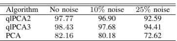
Figure 4 displays the optimal spline transformation of variable 6 from a two dimensional qlPCA on cilinder data without noise. This plot is the typical one among the twelve transformations plots. This type of logarithmic shaped plots was, as expected, the most commonly obtained among the twelve transformation plots. However, an exception - trans-formation of variable twelve - was observed, as it can be seen in Figure 5.
0 2 4 6 8 10 12
0 1 2 3 4 5 6 7 8
Component
Eigenvalue
Two−dimensional qlPCA, two interior knots
0 2 4 6 8 10 12
0 1 2 3 4 5 6 7 8
Component
Eigenvalue
[image:8.595.61.279.270.450.2]Three−dimensional qlPCA, two interior knots
Fig. 3. Scree plot from a two and three dimensional qlPCA on cilinder data with25%noise level. On the y-axis are the eigenvalues of the correlation matrix of the transformed variables.
0 0.02 0.04 0.06 0.08 0.1 0.12 0.14 −2
−1.5 −1 −0.5 0 0.5 1 1.5 2
Variable
Transformed variable
Optimal linear spline transformation on var. 6, three interior knots
Fig. 4. Optimal spline transformations with three interior knots of variable 6 from a two dimensional qlPCA on cilinder data without noise.
Further inspection of this variable shows that the interior knots are placed at 3.85, 10.32 and 25.38 (the quartiles) and that its maximum is 6498.7. This is an example where an al-ternative knot placement could have improved the variable’s
IAENG International Journal of Applied Mathematics, 41:4, IJAM_41_4_14
[image:8.595.311.537.493.676.2]transformation.
0 20 40 60 80 100
0 0.2 0.4 0.6 0.8 1 1.2 1.4 1.6 1.8 2
Variable
Transformed variable
Optimal linear spline transformation on var. 12, three interior knots
Fig. 5. Optimal spline transformations with three interior knots of variable 12 from a two dimensional qlPCA on cilinder data without noise.
VII. CONCLUSION
A new approach on Nonlinear Principal Components Anal-ysis, so-called quasi-linear PCA (qlPCA) was presented in detail in this paper. The qualification quasi emphasize that it refers to the use of linear splines. QlPCA algorithm uses alternating least squares to minimize a suitable objective loss function. It consists of two phases iteratively alternated until convergence is reached, an optimal quantification phase and a estimation of object scores phase.
Nonlinear PCA techniques usually report its solution with relational measures between the nonlinear transformed vari-ables obtained after convergence and the associated objects scores. Considering low order splines some relations between nonlinear principal components and the original variables can be revealed. Optimal transformations are explicitly known after convergence and it was shown that optimization over linear splines have several advantages. It allows projecting new observations onto the nonlinear principal components’ space and reconstruction the original observations. A new concept was also defined - piecewise loadings - as (piece-wise) correlations between nonlinear principal components and the original variables.
QlPCA recovers a spline based algorithm designed for cat-egorical variables (CATPCA) and introduces continuous vari-ables into the framework without the need for a discretization process. It should be emphasized that the proposed algorithm is not intended to be a competitor of CATPCA but rather a different approach.
Nonlinear PCA’s most known approaches among re-searchers dealing with continuous variables are autoasso-ciative neural networks, principal curves and manifolds, kernel approaches or the combination of these [3]. Therefore, comparisons studies with qlPCA will be taken.
Applying qlPCA involves trying out different options regarding spline’s order and the number of interior knots. Researchers are invited to try it out using a MATLAB GUI (Graphical User Interface) that can be obtained from the correspondent author.
REFERENCES
[1] W. Krazanowski and F. Marriott,Multivariate Analysis Part I - Distri-butions, Ordination and Inference, Edward Arnold, 1994.
[2] B. Scho¨olkopf, A. Smola and M¨uller, “Nonlinear component analysis as a kernel eigenvalue problem,”Neural Computation, vol. 10, pp. 1299-1319, 1998.
[3] U. Kruger, J. Zhang and Lei Xie, “Developments and Applications of Nonlinear Principal Component Analysis - a Review,” in: Principal Manifolds for Data Visualization and Dimension Reduction 2007, pp. 1-43.
[4] J. Meulman, A. Kooij and W. Heiser, “Principal Components Analysis with Nonlinear Optimal Scaling Transformations for Ordinal and Nom-inal Data,” inThe Sage Handbook of Quantitative Methodology for the Social Sciences 2004, pp. 49-70.
[5] N. Lavado and T. Calapez, “Quasi-Linear PCA: Low Order Spline’s Approach to NonLinear Principal Components”, inLecture Notes in En-gineering and Computer Science: Proceedings of The World Congress on Engineering 2011, WCE 2011, 6-8 July, 2011, London, U.K., pp. 360-364.
[6] A. Gifi,Nonlinear Multivariate Analysis, Wiley, 1991. [7] C. de Boor,A Practical Guide to Splines, Springer, 1978. [8] L. Schumaker,Spline Functions: Basic Theory, Wiley, 1981. [9] J. Ramsay, “Monotone Regression Splines in Action,”Statistical
Sci-ence, vol. 3, pp. 425-461, 1988.
[10] S. Winsberg and J. Ramsay, “Monotone spline transformations for dimension reduction,”Psychometrika, vol. 48, pp. 575-595, 1983. [11] G. Michailidis and J. De Leeuw, “The GIFI system of descriptive
multivariate analysis,”Statist. Sci., vol. 13, pp. 307-336, 1998. [12] M. Linting, J. Meulman, P. Groenen and A. Van der Kooij, “Nonlinear
principal components analysis: Introduction and application” Psycho-logical Methods, vol.12, pp. 336-358, 2007.
[13] J. De Leeuw and J. Van Rijckevorsel, “Beyond Homogeneity Analy-sis,” in:Component and Correspondence Analysis: Dimension Reduc-tion by FuncReduc-tional ApproximaReduc-tion 1988, pp. 55-80.
[14] J. Jackson,A User’s Guide to Principal Components, Wiley, 1991.
![Figure 1 displays the family of I-splinesdefined onsplineIt also displays an example of the images obtained by eachof the three functions (two basis functions and one spline)for a value ofI and2(0 of degree one [0, 1] with one interior knot at the median](https://thumb-us.123doks.com/thumbv2/123dok_us/386597.536172/3.595.76.253.183.324/displays-splinesdened-onsplineit-displays-obtained-functions-functions-interior.webp)