Maximal Order Block Method For The Solution
Of Second Order Ordinary Differential Equations
Oluwaseun Adeyeye and Zurni Omar
Abstract—Block methods have been seen to be an adequate numerical method for finding the approximate solution to second order ordinary differential equations. Thus, this article presents a block method of maximal order for the direct solution of second order initial and boundary value problems. Taylor series expansion approach is adopted for the derivation of the block methods. From the numerical results obtained, this new block method performs better than previous numerical methods in existence in terms of accuracy, when compared to the exact solution of the numerical problems considered.
Index Terms—Maximal Order, Block Method, Second Order, Initial Value Problems, Boundary Value Problems.
I. INTRODUCTION
Mathematical models have been observed to birth second order ordinary equations either as initial or boundary value problems when it comes to modelling real life situations. Some of these real life models include models for beam deflection and deformation, transmission of heat, temperature distribution across a rod, amongst others [1], [2]. The need to adopt numerical solutions for obtaining an approximate solution of these second order ordinary differential equations is expedient. This is due to the condition that sometimes these ordinary differential equations have more than one solution, or the solution may not exist.
Quite a number of scholars have proposed numerical and ap-proximate methods for the solution of second order ordinary differential equations of the form
y00=f(x, y, y0). (1)
Some authors who have discussed finding approximate solu-tions to (1) with initial condisolu-tions imposed include [3], [4], [5], while the numerical solution when boundary conditions were imposed include the work of [1], [6] and [7].
However, this paper intends to explore the simultaneous solutions of both initial and boundary value problems using the same block method. Although, this approach has been explored by [7] and [8], however, none this work presented a method of maximal order2k+ 2.
Hence, this paper presents ak-step second derivative (k= 3) method to numerically approximate (1) and the numerical results obtained were compared with the results from the previously existing method in literature of equal order despite being of higher step-lengths.
The sections of this paper is arranged as follows; Section 2 presents the methodology, Section 3 shows the basic
Manuscript received December 08, 2015; revised June 22, 2016. Corresponding Author: O. Adeyeye is a PhD candidate at Department of Mathematics, School of Quantitative Sciences, Universiti Utara Malaysia, Sintok, Kedah, Malaysia, e-mail:adeyeye [email protected]
Z. Omar is a Professor of Numerical Analysis at Department of Mathe-matics, School of Quantitative Sciences, Universiti Utara Malaysia, Sintok, Kedah, Malaysia, e-mail:[email protected]
properties of the method while Section 4 will display the results to the numerical problems considered, and Section 5 concludes this paper.
II. METHODOLOGY
The first step entails the derivation of the3−step discrete scheme and its corresponding derivatives. Consider the fol-lowing expression for deriving the discrete scheme.
yn+3 =α0yn+α1yn+1+ 3
X
j=0
βjfn+j+
3
X
j=0
λjfn0+j (2)
which can also be expressed as
yn+3=α0yn+α1yn+1
+ (β0fn+β1fn+1+β2fn+2+β3fn+3) + λ0fn0 +λ1fn0+1+λ2fn0+2+λ3fn0+3
(3)
Using Taylor series expansion to expand individual terms in (3 )and substituting back gives the following matrix representationAx=B as:
1 1 0 0 0 0 0 0 0 0
0 h 0 0 0 0 0 0 0 0
0 (h2!)2 1 1 1 1 0 0 0 0
0 (h3!)3 0 h 2h 3h 1 1 1 1
0 (h4!)4 0 (h2!)2 (22!h)2 (32!h)2 0 h 2h 3h
0 (h5!)5 0 (h3!)3 (2h3!)3 (33!h)3 0 (h2!)2 (2h2!)2 (32!h)2 0 (h6!)6 0 (h4!)4 (2h4!)4 (34!h)4 0 (h3!)3 (2h3!)3 (33!h)3 0 (h7!)7 0 (h5!)5 (2h5!)5 (35!h)5 0 (h4!)4 (2h4!)4 (34!h)4 0 (h8!)8 0 (h6!)6 (2h6!)6 (36!h)6 0 (h5!)5 (2h5!)5 (35!h)5 0 (h9!)9 0 (h7!)7 (2h7!)7 (37!h)7 0 (h6!)6 (2h6!)6 (36!h)6
×(α0, α1, β0, β1, β2, β3, λ0, λ1, λ2, λ3)T
=
1,3h,(32!h)2,(33!h)3,(3h4!)4,(35!h)5,(3h6!)6,(37!h)7,(38!h)8,(3h9!)9 T
and using matrix inverse approach, the following values are obtained
(α0, α1, β0, β1, β2, β3, λ0, λ1, λ2, λ3)
T
= (−2,3,
1961h2
9072 , 263h2
168 , 365h2
336 , 599h2
4536 , 131h3
3780 ,− 103h3
1680 ,
−71h
3
840 ,− 349h3
15120)
T (4)
which gives the following method after substituting back in (3)
yn+3=−2yn+ 3yn+1+
h2
9072(1961fn+ 14202fn+1
+ 9855fn+2+ 1198fn+3) + h3 15120(524f
0
n−927f
0
n+1
−1278fn0+2−349fn0+3) (5)
The next group of methods required is the additional meth-ods for the discrete scheme and the derivatives. The same
IAENG International Journal of Applied Mathematics, 46:4, IJAM_46_4_03
procedure is followed as that of (5) and the methods are given to be:
yn+2=−yn+ 2yn+1+ h
2
9072(908fn+ 6183fn+1 + 1836fn+2+ 145fn+3) + h
3
15120(233f 0
n
−1044fn0+1−1161fn0+2−58fn0+3), yn0 = 1h(−yn+yn+1) +
h
272160(−78076fn−3512fn+1
−19548fn+2−3329fn+3) + h
2
90720(−2597f 0
n
+ 11268fn0+1+ 4005fn0+2+ 274fn0+3), yn0+1= h1(−yn+yn+1) +
h
272160(25319fn+ 91638fn+1 + 16497fn+2+ 2626fn+3) + h
2
90720(1252f 0
n
−11709fn0+1−3258fn0+2−215fn0+3), yn0+2= h1(−yn+yn+1) +
h
272160(28964fn+ 224073fn+1 + 148932fn+2+ 6271fn+3) + h
2
90720(1531f 0
n
−2556fn0+1−12411fn0+2−494fn0+3), yn0+3= h1(−yn+yn+1) +
h
272160(34919fn+ 260118fn+1 + 275697fn+2+ 109666fn+3) + h
2
90720(2020f 0
n
+ 4707fn0+1+ 10566fn0+2−4343fn0+3)
(6) Combining equations (5) and (6) in matrix form gives:
−3 0 1 0 0 0
−2 1 0 0 0 0
−1
h 0 0 0 0 0
−1
h 0 0 1 0 0
−1
h 0 0 0 1 0
−1
h 0 0 0 0 1
yn+1
yn+2
yn+3
yn0+1 yn0+2
yn0+3
= A0 A1 A2 A3 A4 A5 (7) where
A0=−2yn+ h
2
9072(1961fn+ 14202fn+1+ 9855fn+2 +1198fn+3) + h
3
15120(524f 0
n−927fn0+1−1278fn0+2
−349fn0+3)
A1=−yn+ h
2
9072(908fn+ 6183fn+1+ 1836fn+2 +145fn+3) + h
3
15120(233f 0
n−1044fn0+1−1161fn0+2
−58fn0+3)
A2=−yn0 −1hyn+ h
272160(−78076fn−3512fn+1
−19548fn+2−3329fn+3) + h
2
90720(−2597f 0
n+ 11268fn0+1 +4005fn0+2+ 274fn0+3)
A3=−1hyn+272160h (25319fn+ 91638fn+1 +16497fn+2+ 2626fn+3) + h
2
90720(1252f 0
n−11709fn0+1
−3258fn0+2−215fn0+3)
A4=−1hyn+272160h (28964fn+ 224073fn+1 +148932fn+2+ 6271fn+3) + h
2
90720(1531f 0
n−2556fn0+1
−12411fn0+2−494fn0+3)
A5=−1hyn+272160h (34919fn+ 260118fn+1 +275697fn+2+ 109666fn+3) + h
2
90720(2020f 0
n
+4707fn0+1+ 10566fn0+2−4343fn0+3)
and using matrix inverse approach again, the following expressions are obtained:
yn+1=yn+hyn0 + h2
272160(78076fn+ 35127fn+1 + 19548fn+2+ 3329fn+3) + h
3
90720(2597gn
−11268gn+1−4005gn+2−274gn+3), yn+2=yn+ 2hy0n+
h2
8505(5731fn+ 7992fn+1 + 2943fn+2+ 344fn+3) + h
3
2835(206gn
−900gn+1−468gn+2−28gn+3), yn+3=yn+ 3hy0n+ h
2
1120(1206fn+ 2187fn+1 + 1458fn+2+ 189fn+3) + h
3
1120(135gn−486gn+1
−243gn+2−36gn+3), y0n+1=yn0 + h
18144(6893fn+ 8451fn+1+ 2403fn+2 + 397fn+3) + h
2
30240(1283gn−7659gn+1
−2421gn+2−163gn+3), y0n+2=yn0 + h
567(223fn+ 540fn+1+ 351fn+2+ 20fn+3) +945h2 (43gn−144gn+1−171gn+2−8gn+3), y0
n+3=yn0 +224h (93fn+ 243fn+1+ 243fn+2+ 93fn+3) +1120h2 (57gn−81gn+1+ 81gn+2−57gn+3).
(8) Equation (8) gives the expected family of methods needed to approximate boundary value problems in the form of (1) above.
III. PROPERTIES OF THEBLOCKMETHOD
As conventionally known, a linear multistep method is convergent iff it is consistent and zero-stable [9]. Hence, considering the linear operator associated with equation(2)
is defined as
L[y(x);h] =
k
X
j=0
αjyn+j− k
X
j=0
βjfn+j+ k
X
j=0
λjfn0+j (9)
Expandingyn+j,fn+j andfn0+j, we obtain the equation of the following form
L[y(x);h] =C0y(xn)+C1hy1(xn)+· · ·+Cphpyp(xn)+. . .
The method is said to be of order p if C0 = C1 =· · · =
Cp =Cp+1= 0,Cp+2 6= 0andCp+2 is the error constant,
where m is the order of the differential equation under consideration.
Likewise, considering the lineark-step method, the order p is said to be maximal ifp= 2k+ 2[10].
Hence, the block method displays uniform maximal order p= (8,8,8,8,8,8)T with error constant
C10= 50803200359 , 17 793800, 27 627200, 313 25401600, 13 793800, 9 313600 T . Definition 3.1 (10): Given a linear k-step method, the orderpis said to be maximal if p= 2k+ 2.
Definition 3.2 (7): A linear multistep method isconsistent if it has orderp≥1.
To analyze the method for zero stability, the block method
(12)is normalized to give the first characteristic polynomial as
ρ(R) =det RA0−A1
=R2(R−1)
where A0 is the identity matrix of dimension 3 and A1 is
given by
A1=
0 0 1
0 0 1
0 0 1
IAENG International Journal of Applied Mathematics, 46:4, IJAM_46_4_03
The roots ofρ(R) = 0 satisfy|Rj| ≤1, j= 1,2,3.
Hence, the block method is convergent since it is both consistent and zero-stable.
The region of absolute stability is determined by obtaining the stability polynomial from
det
" k
X
i=0
Aiqk−i+zm k
X
i=0
Biqk−i+zm+1 k
X
i=0
Ciqk−i
#
(10) wherez=λhandmis the order of the differential equation. Hence, the stability polynomial for the block method is gotten as
R(q) =−23520029q6z9 +36400q6z8 +q19606z7 −179711693440q6z6 +q632z5 +432240q6z4 −9q6z3
28 +
649q6z2
1008 +
43q3z9
313600+ 277q3z8
134400 +56931360q3z7 +1971431693440q3z6 +791280q3z5 +31872240q3z4 −27112q3z3
+38871008q3z2 +q3
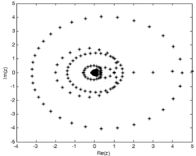
[image:3.595.69.265.340.496.2]Plotting the roots of the stability polynomial in boundary locus approach displays the region of absolute stability as shown below.
Figure 1: Region of Absolute Stability for (8)
IV. NUMERICALRESULTS ANDDISCUSSION
The following numerical problems are considered for the purpose of showing the accuracy of the new method when compared to previously existing methods
1) Consider the general second order initial value problem from [11]
y00+6
xy 0+ 4
x2y= 0, y(1) = 1, y
0(1) = 1, h=0.1 32
(11) with exact solution
y(x) = 5 3x−
2 3x4
2) Consider the special second order initial value problem from [12]
y00−100y= 0, y(0) = 1, y0(0) =−10, h= 0.01
(12) with exact solution
y(x) =e−10x
3) Consider the non-linear second order initial value prob-lem from [13]
y00−x(y0)2= 0, y(0) = 1, y0(0) = 1
2, h= 0.1 (13)
with exact solution
y(x) = 1 +1 2ln
2 +x
2−x
4) Consider the linear second order boundary value prob-lem from [6]
y00=y+ cosx, y(0) = 0, y(1) = 1, h= 0.125
(14) with exact solution
y(x) =−3 cosh 1 + 3 sinh 1 + cos 1 + 2
4 sinh 1 e
x+
3 cosh 1 + 3 sinh 1−cos 1−2
4 sinh 1 e
−x−cosx
2
5) Consider the general second order boundary value problem from [6]
y00=y0−e(x−1)−1, y(0) = 0, y(1) = 0, h= 0.1
(15) with exact solution
y(x) =x1−e(x−1)
6) Consider the boundary value problem from [6]
y00+xy= 3−x−x2+x3
sinx+ 4xcosx,
y0(0) =−1, y0(1) = 2 sin 1 (16)
with exact solution
y(x) = (x2−1) sinx
7) Consider the oscillatory nonlinear system of initial value problems studied by [14]
y100=−4x2y1− 2y2
p
y2 1+y22
, y1(x0) = 1, y10(x0) = 0,
y200=−4x2y2+ 2y1
p
y2 1+y22
, y2(x0) = 0, y20(x0) = 0
(17)
whose exact solutions are given byy1(x) =cosx2and
y2(x) =sinx2
8) Consider the linear system of second order boundary value problems studied by [15]
d2u 1
dx2 + (2x−1)
du1
dx + cosπx du2
dx =f1(x) d2u
2
dx2 +xu1=f2(x) 0≤x≤1 (18)
where
f1(x) =−π2sinπx+ (2x−1)(π+ 1) cosπx
f2(x) = 2 +xsinπx
subject to boundary conditions
u1(0) =u1(1) = 0, u2(0) =u2(1) = 0
whose exact solutions are
u1(x) = sinπx and u2(x) =x2−x
IAENG International Journal of Applied Mathematics, 46:4, IJAM_46_4_03
9) (Bessel’s IVP) Consider the Bessel differential equa-tion that was solved by [16] and also [17]
x2y00+xy0+ x2−0.25y= 0, x∈[1,8] (19) subject to initial conditions
y(1) =
r
2
pisin 1'0.671397071418031
whose exact solutions are
y0(1) = 2 cos 1−sin 1
2∗pi '0.0954005144474746
[image:4.595.58.295.55.196.2]The results and comparison of error of the problems considered are given in the tables below.
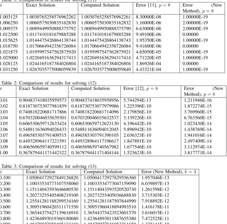
Table 1: Comparison of results for solving (11)
x Exact Solution Computed Solution Error [11],p= 8 Error (New
Method),p= 8
1.003125 1.0030765258576962262 1.0030765258576962261 8.30000E-08 1.00000E-19 1.006250 1.0060575030835162830 1.0060575030835162832 1.16000E-06 2.00000E-19 1.009375 1.0089449950888375792 1.0089449950888375790 6.63000E-06 2.00000E-19 1.012500 1.0117410181679885288 1.0117410181679885288 9.49100E-06 0.00000 1.015625 1.0144475426864138744 1.0144475426864138743 1.95350E-06 1.00000E-19 1.018750 1.0170664942356726084 1.0170664942356726084 9.41600E-06 0.00000 1.021875 1.0195997547562875920 1.0195997547562875921 4.65050E-05 1.00000E-19 1.025000 1.0220491636294317413 1.0220491636294317414 4.71220E-05 1.00000E-19 1.028125 1.0244165187384026804 1.0244165187384026804 1.86926E-04 0.00000 1.031250 1.0267035775008059839 1.0267035775008059840 4.43321E-04 1.00000E-19
Table 2: Comparison of results for solving (12)
x Exact Solution Computed Solution Error [12], p= 8 Error (New
Method), p= 8
0.01 0.904837418035959573 0.904837418035958956 5.744294E-13 1.211946E-16 0.02 0.818730753077981859 0.818730753077979986 1.225396E-10 1.872274E-15 0.03 0.740818220681717866 0.740818220681714096 2.179856E-10 3.769960E-15 0.04 0.670320046035639301 0.670320046035632537 3.139226E-10 6.763560E-15 0.05 0.606530659712633424 0.606530659712623130 4.196442E-10 1.023430E-14 0.06 0.548811636094026433 0.548811636094012045 5.896942E-10 1.438769E-14 0.07 0.496585303791409515 0.496585303791390105 2.036323E-10 1.941016E-14 0.08 0.449328964117221591 0.449328964117196617 1.847891E-10 2.497409E-14 0.09 0.406569659740599112 0.406569659740567982 1.677546E-10 3.112974E-14 1.00 0.367879441171442322 0.367879441171404144 1.523623E-10 3.817771E-14
Table 3: Comparison of results for solving (13)
x Exact Solution Computed Solution Error (New Method),k= 3
0.100 1.05004172927849126820 1.05004172927829556360 1.957046E-13 0.200 1.10033534773107558060 1.10033534773047159090 6.039897E-13 0.300 1.15114043593646680530 1.15114043593520520730 1.261598E-12 0.400 1.20273255405408219100 1.20273255405036688830 3.715303E-12 0.500 1.25541281188299534160 1.25541281187507644990 7.918892E-12 0.600 1.30951960420311171550 1.30951960418894993510 1.416178E-11 0.700 1.36544375427139616910 1.36544375423523601570 3.616015E-11 0.800 1.42364893019360180680 1.42364893011887655380 7.472525E-11 0.900 1.48470027859405174160 1.48470027846053761650 1.335141E-10 1.000 1.54930614433405484570 1.54930614390236873630 4.316861E-10
IAENG International Journal of Applied Mathematics, 46:4, IJAM_46_4_03
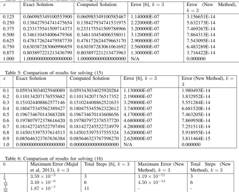
[image:4.595.54.519.240.699.2]Table 4: Comparison of results for solving (14)
x Exact Solution Computed Solution Error [6], k= 3 Error (New Method), k= 3
0.125 0.060985349100553900 0.060985349100585467 1.140000E-07 3.156651E-14 0.250 0.138427934741475654 0.138427934741531975 2.220000E-07 5.632173E-14 0.375 0.233175541509714373 0.233175541509788966 3.200000E-07 7.469267E-14 0.500 0.346110454006479368 0.346110454006558011 3.120000E-07 7.864313E-14 0.625 0.478172624479587739 0.478172624479663170 2.900000E-07 7.543095E-14 0.750 0.630387283060996859 0.630387283061061692 2.560000E-07 6.483289E-14 0.875 0.803897221213436799 0.803897221213473963 1.300000E-07 3.716422E-14 1.000 1.000000000000000000 1.000000000000000000 N/A 0.000000
Table 5: Comparison of results for solving (15)
x Exact Solution Computed Solution Error [6],k= 3 Error (New Method),k= 3
0.1 0.059343034025940089 0.059343034025920284 1.130000E-07 1.980493E-14 0.2 0.110134207176555682 0.110134207176517352 2.190000E-07 3.832952E-14 0.3 0.151024408862577146 0.151024408862521633 3.290000E-07 5.551284E-14 0.4 0.180475345562389427 0.180475345562322612 3.740000E-07 6.681520E-14 0.5 0.196734670143683288 0.196734670143608656 4.170000E-07 7.463205E-14 0.6 0.197807972378616420 0.197807972378537720 4.680000E-07 7.869950E-14 0.7 0.181427245522797494 0.181427245522724979 4.280000E-07 7.251511E-14 0.8 0.145015397537614513 0.145015397537555324 3.620000E-07 5.918955E-14 0.9 0.085646323767636384 0.085646323767598270 2.620000E-07 3.811464E-15 1.0 0.000000000000000000 0.000000000000000000 N/A 0.000000
Table 6: Comparison of results for solving (16) h Maximum Error (Majid
et al, 2013),k= 3
Total Steps [6], k= 3 Maximum Error (New Method),k= 3
Total Steps (New Method),k= 3 1
8 3.59×10
−5 3 1.19×10⁻¹¹ 3
1
16 3.49×10
−6 6 4.50×10⁻¹⁴ 6
1
32 1.87×10
−7 11 -
-1
64 1.28×10
−8 22 -
-1
128 7.76×10
−10 43 -
-Table 7: Comparison of results for solving (19)
N Maximum Error [16] Maximum Error [17] Maximum Error
(New Method)
67 1.14×10⁻⁹ 7.11×10⁻⁷ 1.46×10⁻¹⁰
82 3.50×10⁻¹⁰ 9.26×10⁻⁸ 3.30×10⁻¹¹ 97 1.30×10⁻¹⁰ 87.8×10⁻⁹ 9.31×10⁻¹² 112 5.50×10⁻¹¹ 1.12×10⁻¹⁰ 3.51×10⁻¹² 125 2.90×10⁻¹¹ 2.71×10⁻¹¹ 1.44×10⁻¹²
IAENG International Journal of Applied Mathematics, 46:4, IJAM_46_4_03
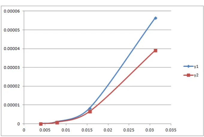
Figure 2 shows the maximum error for Problem (17) plotted against various step sizes h=21i, i= 5, . . . ,8
Figure 2: Step sizes versus Maximum Error for Problem (17)
[image:6.595.44.389.394.601.2]Figure 3 shows the maximum error for problem (18) plotted against increasing number of iterations N = 10,20,30,40,50
Figure 3: Number of Iterations versus Maximum Error for Problem (18)
IAENG International Journal of Applied Mathematics, 46:4, IJAM_46_4_03
V. CONCLUSION
This work presents a three-step method of maximal order for approximating the solution of second order initial and boundary value problems. To show the superiority of the maximal order block method introduced, certain numerical examples were considered. These included the solution of system of linear initial and boundary value problems, and the results were compared to previously existing methods of either equal order or equal steplength. From the results displayed in the tables above, the maximal order block method was seen to display more favourable results and also in accordance to literature, the accuracy increased as the number of iterations (N) increased and as the step-size (h) reduced when adopted for the solution of the system of ordinary differential equations. This is further justified as seen in Table 6, where the maximum error of the maximal order block method ath−value of 161 is giving faster convergence than the previously existing method even at a smaller h−value of 1281 . Therefore, the maximal order block method can be adopted for the solution of equations in the form of (1) or a system of (1) with either initial or boundary conditions imposed.
REFERENCES
[1] P. P. See, Z. A. Majid, and M. Suleiman, “Solving nonlinear two point boundary value problem using two step direct method,” Journal of Quality Measurement and Analysis, vol. 7, no. 1, pp. 127-138, 2011. [2] S. Islam, I. Aziz, and B. Sarler, “The numerical
so-lution of second-order boundary-value problems by collocation method with the Haar wavelets,” Mathe-matical and Computer Modelling, vol. 52, no. 9-10, pp. 1577-1590, 2010.
[3] D. O. Awoyemi, E. A. Adebile, A. O. Adesanya, and T. A. Anake, “Modified block method for the direct solution of second order ordinary differential equa-tions,” International Journal of Applied Mathematics and Computation, vol. 3, no. 3, pp. 181-188, 2011. [4] A. A. James, A. O. Adesanya, and S. Joshua,
“Contin-uous block method for the solution of second order ini-tial value problems of ordinary differenini-tial equation.” International Journal of Pure and Applied Mathemat-ics, vol. 83, no. 3, pp. 405-416, 2013.
[5] Z. Omar, and J. O. Kuboye, “Derivation of block methods for solving second order ordinary differential equations directly using direct integration and col-location approaches,” Indian Journal of Science and Technology, vol. 8, no. 12, 2015.
[6] Z. A. Majid, M. M. Hasni, and N. Senu, “Solving second order linear dirichlet and neumann boundary value problems by block method,” IAENG Interna-tional Journal of Applied Mathematics, vol. 43, no. 2, pp. 71-76, 2013.
[7] S. N. Jator, and J. Li, “Solving two-point boundary value problems by a family of linear multistep meth-ods,”Neural, Parallel and Scientific Computations, vol. 17, no. 2, pp. 135-146, 2009.
[8] A. M. Sagir, “A family of zero stable block integrator for the solutions of ordinary differential equations,” World Academy of Science, Engineering and Technol-ogy, vol. 7, no. 6, pp. 751-756, 2013.
[9] S. O. Fatunla, Numerical methods for initial value problems in ordinary differential equations, Boston, New York: Academic Press, 1988.
[10] J. C. Butcher, Numerical methods for ordinary differ-ential equations, New York: John Wiley & Sons Inc, 2008.
[11] A. M. Badmus, “A new eighth order implicit block algorithms for the direct solution of second order ordinary differential equations,” American Journal of Computational Mathematics, vol. 4, no. 4, pp. 376-386, 2014.
[12] J. O. Kuboye, and Z. Omar, “Solving second order or-dinary differential equations directly by uniform order eight block method,”Far East Journal of Mathematical Sciences, vol. 98, no. 3, pp. 315-332, 2015.
[13] T. A. Anake, D. O. Awoyemi, and A. O. Adesanya, “One-step implicit hybrid block method for the direct solution of general second order ordinary differential equations,” IAENG International Journal of Applied Mathematics, vol. 42, no. 4, pp. 224-228, 2012. [14] N. A. Yahya, M. Awang, and A. Ibrahim, “Embedded
5(4) pair implicit 2-step hybrid method for solving spe-cial second-order initial value problems,” In Human-ities, Science and Engineering Research (SHUSER), 2012 IEEE Symposium, 299-304. 2012
[15] M. El-Gamel, “Sinc-collocation method for solving linear and nonlinear system of second-order boundary value problems,”Applied Mathematics, vol. 3, no. 11, pp. 1627-1633, 2012.
[16] F. F. Ngwane, and S. N., Jator, “Solving the Telegraph and Oscillatory Differential Equations by a Block Hybrid Trigonometrically Fitted Algorithm,” Interna-tional Journal of Differential Equations, vol. 2015, no. 347864, pp. 1-15, 2015.
[17] J. Vigo-Aguiar, and H. Ramos, “Variable stepsize implementation of multistep methods for y00 =
f(x, y, y0),” Journal of Computational and Applied Mathematics, vol. 192, no. 1, pp. 114-131, 2006.