Bayesian modelling and analysis of utility based maintenance for repairable systems

(1)

Bayesian Modelling and Analysis of

Utility-based Maintenance for

Repairable Systems

A thesis submitted to the University of Dublin, Trinity College

in partial fulfillment of the requirements for the degree of

Doctor of Philosophy

Department of Statistics, Trinity College Dublin

September 2016

(2)

(3)

(4)

(5)

Declaration

I declare that this thesis has not been submitted as an exercise for a degree at this

or any other university and it is entirely my own work.

I agree to deposit this thesis in the University’s open access institutional repository

or allow the Library to do so on my behalf, subject to Irish Copyright Legislation and

Trinity College Library conditions of use and acknowledgement.

The copyright remains solely with the author, Shuaiwei Zhou.

Shuaiwei Zhou

(6)

(7)

Abstract

This thesis focuses on modelling and inference for maintenance systems for the

pur-pose of utility optimisation. Providing standardised notation throughout, we first

demonstrate the motivation for investigating the problem of modelling and inference

for maintenance systems and briefly state the problems which are to be explored. The

definitions and terminology, which are also used within the general domains of science

and engineering, have been presented in terms of statistical representation.

We propose a Bayesian method to optimise the utility of a two phase maintenance

system sequentially by dynamic programming method. In particular, the parameters

of the failure distribution for the system of interest are analysed within the Bayesian

framework. Utility-based maintenance is modelled in several modified models,

in-cluding imperfect preventive maintenance, time value of money effect in maintenance,

maintenance for systems with discrete failure time distributions, maintenance for

par-allel redundant systems, of which all follow numerical examples. A hybrid approach

combining myopic and dynamic programming method is proposed to solve multi-phase

maintenance systems.

The Bayesian dynamic programming is carried out through the gridding approach

to solve the issue arising from nested series of maximisations and integrations over

a highly non-linear space. The core of gridding method, the increment is studied

extensively. We also utilise and modify the approach proposed by Baker (2006) to

analyse the effect of risk aversion on the variability of system in cash flows.

The potential generalisation of the current models has been discussed and the future

work concerning complicated models and efficient computation methods have also been

(8)

(9)

Acknowledgements

I would like to express my utmost and sincere gratitude to my two wonderful

super-visors, Professor Simon P. Wilson and Professor Brett Houlding, for their invaluable

guidance and constant devotion to me during my PhD research. No matter how stupid

the questions I asked or how na¨ıve I was, they were always extremely patient to explain

and explore potential ideas with me.

Within the discipline of statistics, I would like acknowledge the kind help and

interesting discussions with the professors in our department and beyond, in particular

Myra O’Regan, John Hasslet, Eamonn Mullins and Elizabeth Heron. My memorable

PhD journey has been thankfully shared with fellow researchers who are Jason Wyse,

Louis Aslett, Susanne Schimitz, Arnab Bhattacharya, Tiep Mai, Arthur White, Gernot

Roetzer and Angela McCourt. I have been fortunate to have wonderful friendships

with Sean O’Riordain, Cristina De Persis, Thinh Doan, Donnacha Bolger and Shane

O’Meachair. My appreciation also goes to Charles McLaughlin and Michael Kelly with

their generous help during my PhD life in Ireland.

I am also indebted to my parents, and my brother and his wife, for their incredible

encouragement and support. Xiaoyao and Xiaonan, who burst onto the scene during

my undergraduate and postgraduate time, makes me proud of being a happy uncle.

The generous support of a four-year scholarship by the China Scholarship Council

and a three-year studentship by the University of Dublin made it all feasible.

Shuaiwei Zhou

Trinity College, Dublin

(10)

(11)

Abbreviations

ARA Absolute Risk Aversion

CARA Constant Absolute Risk Aversion

CBM Condition-based Maintenance

CDF Cumulative Distribution Function

CE Certainty Equivalent

CHF Cumulative Hazard Function

CM Corrective Maintenance

CR Cost Rate

CRRA Constant Relative Risk Aversion

DARA Decreasing Absolute Risk Aversion

DP Dynamic Programming

DRRA Decreasing Relative Risk Aversion

GA Genetic Algorithm

H-M-DP Hybrid Myopic Dynamic Programming

IARA Increasing Absolute Risk Aversion

IID Independent and Identically Distributed

IPM Imperfect Preventive Maintenance

IRRA Increasing Relative Risk Aversion

PDF Probability Density Function

PM Preventive Maintenance

PMF Probability Mass Function

PPM Perfect Preventive Maintenance

RRA Relative Risk Aversion

(12)

(13)

List of Tables

2.1 State Assumptions after Maintenance . . . 17

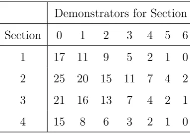
3.1 Number of failed students for a course with 4 sessions and 6 available demonstrators. . . 36

3.2 Dynamic Programming Example: Stage 4. . . 37

3.6 Properties of Utility Functions . . . 49

4.1 Optimal corrective maintenance (CM) time and corresponding expected cost for each chance node based on dynamic programming and myopic methods. Bracketed figures are failure timeTf1 with respect toT ∗ m1 and T_m∗₂, numbers in brackets representing corresponding failure times. . . . 86

4.2 Optimum Perfect Preventive Maintenance (PPM) time through different optimisation objectives,i.e., expected cost and expected utility for each chance node based on dynamic programming method. Bracketed figures are failure time Tf1 with respect to Tm1 and Tm2, numbers in brackets representing corresponding failure times. . . 87

4.3 Optimal perfect preventive maintenance (PPM) time and corresponding expected utility for chance node CN1 by dynamic programming condi-tioning on various risk aversion parameter η of an exponential utility function. . . 88

(18)

5.1 Optimal Imperfect Preventive Maintenance (IPM) time and

correspond-ing expected cost for chance nodesCN1 andCN22 conditioning on

vari-ous PM power parameterβ based on dynamic programming and myopic

methods. . . 97

5.2 Optimal Perfect Preventive Maintenance (PPM) time and corresponding

expected cost rate for chance node CN1 conditioning on various time

effect parameter r based on dynamic programming. . indicates the

cost rate comparison to its previous one. . . 99

5.3 Optimal perfect preventive maintenance (PPM) time and corresponding

expected cost for chance nodeCN1 by dynamic programming

condition-ing on various parameterp of a discrete Weibull failure distribution. . . 102

expected cost rate for each chance node by dynamic programming for

one-unit systems and two-unit redundant parallel systems. Bracketed

figures are failure time Tf1 with respect to Tm1 and Tm2, numbers in

brackets representing corresponding failure times. . . 104

5.5 Optimal Perfect Preventive Maintenance (PPM) time and corresponding

expected cost rate for each chance node by dynamic programming based

on Weibull and gamma failure time assumptions. Bracketed figures are

failure time Tf1 with respect to Tm1 and Tm2, numbers in brackets

rep-resenting corresponding failure times. . . 107

5.6 Optimal Perfect Preventive Maintenance (PPM) time and

correspond-ing expected cost rate of chance nodes CN21 and CN22 for three-phase

maintenance systems based on Hybrid Myopic-Dynamic Programming

and myopic methods. . . 115

5.7 Comparison of optimal perfect preventive maintenance (PPM) time and

corresponding expected cost for each chance node based on different

in-crement parameterδ. Bracketed figures are failure timeTf1 with respect

toTm1 and Tm2, numbers in brackets representing corresponding failure

(19)

expected cost for chance node CN1 conditioning on various increment

parameterδ based on dynamic programming. . . 119

5.9 Optimal perfect preventive maintenance (PPM) time and

correspond-ing expected cost for chance node CN1 conditioning on cost difference

between failure and maintenance based on dynamic programming. . . . 121

expected cost for chance nodeCN1 conditioning on various prior mean

of parameterθ based on dynamic programming. . . 122

5.11 Optimal perfect preventive maintenance (PPM) time and

correspond-ing expected cost for chance node CN1 conditioning on various prior

standard deviation of parameterθ based on dynamic programming. . . 123

expected cost for each chance node by dynamic programming based on

non-Log and Log utility functions. Bracketed figures are failure time

Tf1 with respect toTm1 and Tm2, numbers in brackets representing

(20)

(21)

List of Figures

2.1 Comparison of Weibull Distributions with Different Shape Parameters

η: Probability Density Functions (top-left), Cumulative Distribution

Functions (top-right), Survival Functions (bottom-left), Hazard

Func-tions (bottom-right). . . 11

2.2 Comparison of Gamma Distributions with Different Shape Parameters

η: Probability Density Functions (top-left), Cumulative Distribution

Functions (top-right), Survival Functions (bottom-left), Hazard

Func-tions (bottom-right). . . 13

4.1 Decision Tree for Two-Phase System . . . 56

4.2 Exponential utility functions with various risk-aversion parameter η. . . 59

4.3 Comparison of truncated normals with various mean (left) and

truncat-ing points (right). . . 64

4.4 Expectation ofTf (left) and variance of Tf (right) given θ and κ= 1. . 66

4.5 Prior distribution ofθ: truncated normal distributionN(2, 1) truncated

at 1. . . 66

4.6 Expectation ofθ (left) and variance of θ (right) given a and b=∞. . . 67

4.7 Marginal density of Tf1: fTf1(tf1) =

R

f(tf1|θ)f(θ)dθ. . . 68

4.8 Maintenance Time Optimisation Simplification. . . 72

4.9 Prior distribution of θ (left) and marginal distribution of Tf1 (right) by

the gridding method. . . 74

4.10 Probability of Tf2 conditioning on tf1, i.e., pTf2(tf2|tf1 =i), where i=

0.1, . . . ,6, by the gridding method. . . 75

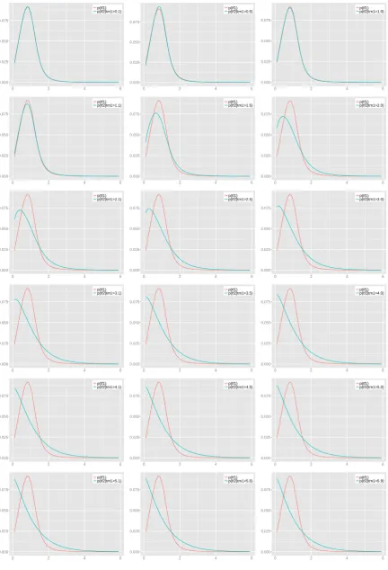
4.11 Comparison ofpTf1(tf1) (red) andpTf2(tf2|tf1 =i) (green), wherei= 0.1,

(22)

4.12 3D scatter plot for maximal probability of Tf2 conditioning on tf1, i.e.,

maxpTf₂(tf2|tf1), with vertical lines for each point. . . 77

4.13 Maximal probability of Tf2 conditioning on tf1, i.e., maxpTf2(tf2|tf1). . 77

4.14 Tf2 that has maximal probability conditioning ontf1,i.e., arg maxpTf₂(tf2|tf1);

corresponding probabilities (rounded to 2 decimals) shown alongside

dots that represent Tf2 which maximise the probabilities given a

spe-cific tf1. . . 78

4.15 Maximal probability ofTf2 and the corresponding Tf2; correspondingtf1

shown alongside dots. . . 79

4.16 Probability of Tf2 conditioning on tf1 > Tm1, i.e., pTf₂(tf2|tf1 > Tm1),

whereTm1 = 0.1, . . . ,6, by the gridding method. . . 80

4.17 Comparison of pTf₁(tf1) (red) and pTf₂(tf2|tf1 > Tm1) (green), where

Tm1 = 0.1, 0.5, 1.0, 1.1, 1.5, 2.0, 2.1, 2.5, 3.0, 3.1, 3.5, 4.0, 4.1, 4.5, 5.0,

5.1, 5.5, 5.9. . . 81

4.18 Expected utilities for two-phase systems at chance nodes CN21, CN22

and CN1 under the dynamic programming method. . . 85

4.19 Expected costs for two-phase systems at chance nodes CN21,CN22 and

CN1 under the dynamic programming method. . . 87

4.20 Risk aversion parameter η on utility. . . 88

4.21 Optimal Maintenance Decision Tree for Two-Phase Systems. . . 89

4.22 Posterior probability density of θ conditioning on Tf1(≤0.5) and Tf1 >

0.5 compared with prior probability density of θ. . . 90

5.1 Comparison of probabilities ofTf2 conditioning on optimalTm1 obtained

through PPM and IPM. . . 95

5.2 Comparison of probabilities of Tf2 conditioning on observed Tf1 and

implemented imperfect preventive maintenance atTm1. . . 96

5.3 Discrete Weibull Probability Mass Functions (top-left: p = 0.01, θ = 2;

top-right: p = 0.1, θ = 2; bottom-left: p = 0.5, θ = 2; bottom-right:

p= 0.9, θ= 2). . . 101

5.4 Marginal Weibull and gamma probabilities of Tf1, pW(tf1) and pG(tf1)

(23)

5.5 Decision tree for three-phase system with sequential problem with

shad-ing indicatshad-ing a range of possible outcomes for the precedshad-ing chance

node; Box DP-1 and DP-2 show the break into two period problems. . 109

5.6 Comparison of probabilities of Tf2 conditioning on varying Tf1 and

op-timalTm1. . . 111

5.7 Posterior probability density of θ conditioning on Tf1 ≤ Tm1(0.5) and

Tf1 > Tm1(0.5) compared with prior probability density ofθ. . . 113

5.8 Expected cost rates at chance node CN21 conditioning on tf1 ≤ Tm1

(top-left: tf1 = 0.1, top-right: tf1 = 0.2, middle-left: tf1 = 0.3,

middle-right: tf1 = 0.4 and bottom-left: tf1 = 0.5; and expected cost rates at

chance node CN22 conditioning on tf1 > Tm1 (bottom-right) under the

H-DP-M method. . . 114

5.9 Optimal Maintenance Decision Tree for Three-Phase Systems . . . 116

5.10 Sensitivity analysis concerning gridding intervals: Compiling time

(top-left); Optimal Maintenance Time (top-right); Expected Cost Rate

(bottom-left); Expected Cost Rate per Compiling Time Unit (bottom-right). . . 120

5.11 Parallel Computing for p(tf2, tf1) . . . 125

6.1 Certainty-Equivalent with the risk-aversion parameterηunder different

(24)

(25)

Chapter 1

Introduction

1.1

Background and Motivation

In the current climate of globalisation, competition as well as varying demands from

stakeholders, increasing pressure on manufacturing performance has been one of the

main driving forces in the growth of manufacturing industries (Tsang, 2002). From this

point of view maintenance is a significant activity in industrial practice, resulting in the

importance of maintenance optimisation. Maintenance aims to combat the inevitable

degradation of systems over their operational lifetime and keep them in working order.

Therefore, maintenance plays an important role in sustaining and improving systems

availability, which in turn affects the productivity of the system of interest.

Recently, more attention has been directed towards improving and optimising

main-tenance in manufacturing systems as inappropriate mainmain-tenance could result in huge

cost and risk (Holmberg et al., 2010). Maintenance costs can reach anywhere between

15% and 70% of production costs (Wang et al., 2008), which also indicates that there

is still a large potential for increasing the productivity in current maintenance

prac-tices. In some industries, a slight improvement in throughput could result in significant

economic impact.

In modern times, the complexity of maintenance systems has increased drastically,

see Duffuaa et al. (2001). This is partly due to modern manufacturing systems which

involve numerous interactions and dependencies between components. It is evident

that analytical and mathematical approaches are limited in solving such complex

(26)

analysis is applied to use accumulating evidence to make advantageous early decisions.

In the context of system engineering, this could help save cost and even improve

sys-tem performance. The Bayesian method of sequential analysis is to make decisions that

minimise the expected value of some loss function which can be viewed as a function

of corresponding inputs and outputs, see DeGroot (1970) and Brockwell and Kadane

(2003). In this thesis, we focus the study on Bayesian sequential analysis applied to

maintenance optimisation of repairable systems.

The study of system maintenance has attracted increasing attention in recent years

because of a need from industry for increasing the reliability and availability of systems

whilst decreasing the associated costs. Percy and Kobbacy (1996) pioneered work in

preventive maintenance modelling from a Bayesian perspective. Damien et al. (2007)

analysed a single item maintenance in a Bayesian semi-parametric setting, which solves

the drawbacks of other models failing to capture the true underlying relationships in

the data. However, their analysis is based on a pre-defined finite time horizon, for

example, see Baker (2010); in other words, the maintenance time phases are pre-defined

which is not practical in reality; in our work, on the contrary, the maintenance time

phases are also pre-defined depending on a particular system but random and flexible,

which meets the maintenance scheduling programme. Nonparametric methods have

also been investigated in system maintenance. Gilardoniet al. (2013) use a

power-law-process parametric method by incorporating the nonparametric maximum likelihood

estimate of an intensity function to estimate the optimal preventive maintenance policy.

However, all these approaches fail to consider sequential maintenance which requires

more complicated modelling and longer computation time.

Maintenance based on prognostics is a prior event analysis and action. By means

of incorporating prognostics into the maintenance decision making process, one could

carry out a maintenance forecast based on known characteristics as well as the

evalua-tion of the significant parameters of the item. With regard to maintenance objectives,

as in most of the literature cost-based optimisation framework is taken (Van Horenbeek

et al., 2010). However, focus should not only be on costs as risk preference is simply

ignored if only cost-oriented objective is taken into account. Utility functions used

to measure risk preferences are ubiquitous in economic research. The little published

(27)

Rao (1993); Keren and Pliskin (2006). In fact, the field of maintenance and reliability

is a suitable area to apply risk-averse policies because there are numerous cash flows

occurring stochastically. A drawback of taking cost per unit time as a criterion of

optimality is that two policies might then be equally attractive, even if for one of them

the annual maintenance spend were much more variable than that for the other. What

might be seen by some as over-maintenance, in the sense that mean cost per unit time is

not minimised, could be optimal as a risk-averse policy, in which the large unscheduled

losses from failure have such a dis-utility that very frequent maintenance is carried out.

Clearly, a policy that minimised cost per unit time would be unsatisfactory for a

main-tenance engineer who could not convince management that periods of high loss were

an unavoidable part of an optimal long-term policy or for an enterprise that could not

survive because of short-term cash flow problems. Thus, extra maintenance activity is

an insurance policy against large losses occurring over a period.

Models and methodologies proposed in this thesis are primarily suited for large

in-dustrial purposes, for example, an automatic manufacturing system, a robotic process,

or a computer server for the non-life essential services, in which cases failure is neither

rare or frequent, maintenance itself is not cheap or trivial, but failure is a considerable

expense, though not exorbitantly so. Hence, this approach is not suitable to apply to

maintenance of systems with very high risk aversion properties, e.g., a nuclear power

facility, an off-shore oil field, or a life support system. It is also not worthwhile applying

to trivial systems where the computational cost of performing this analysis outweighs

any savings.

1.2

Structure and Main Contributions

The overall research goal of this thesis is to develop a utility-based prognostic

mainte-nance optimisation methodology within a Bayesian statistical framework, which uses

historical information and predictions in remaning lifetime of repairable systems.

The following is an overview of the structure of this thesis along with the main

research contributions.

• Chapter 1 introduces the research background and motivation, and briefly

(28)

• Although research background and motivation is given in Chapter 1, Chapter

2 gives a detailed review on maintenance modelling and analyses as well as the

fundamental concepts in systems maintenance, from reliability measures to

clas-sical failure time distributions. We highlight the essential publications which are

highly related to the research questions in this thesis.

• For those beyond the statistical research community, Chapter 3 briefly presents

the Bayesian perspective on modelling, and continues to introduce the

founda-tional concepts of the dynamic programming method as well as utility theory,

which are the maintenance optimisation methodologies in this research.

• Chapter 4 solves the sequential maintenance problem under the policy of perfect

preventive maintenance by a dynamic programming method utilising the idea

proposed by Brockwell and Kadane (2003), whereby a grid is constructed in the

maintenance and failure time space, over which the utility functions of expected

cost per unit time are evaluated. This method has a computation time which is

linear in the number of phases in the sequential problem.

• Chapter 5 extends the previous sequential preventive models to imperfect

preven-tive maintenance, taking account of the time value of money, modelling prevenpreven-tive

maintenance in discrete time setting as well as maintenance for parallel systems,

analysing the effect of failure time distribution assumptions on preventive

mainte-nance time and proposing an adaptive approach to solving multi-phase systems’

maintenance. Sensitivity analysis via the parameters of sequential preventive

maintenance models will also be carried out in the chapter.

• Chapter 6 utilises and modifies the approach proposed by Baker (2006) to

inves-tigate and analyse the effect of risk aversion on the variability of system in cash

flows from a certainty-equivalent point of view.

• Chapter 7 states the major conclusions and contributions of this research and

(29)

Chapter 2

Repairable Systems and

Maintenance

In this chapter we introduce the difference between non-repairable systems and

re-pairable systems, and classify the maintenance policies and review related modelling

methods.

2.1

Repairable Systems

2.1.1

Basic Terminology and Examples

A repairable system is a system that can be restored to an operating condition by some

repair process instead of replacement of the entire system. For example, an automobile

is a repairable system because most failures, such as the inability to start because of

a bad starter, can be fixed without replacing the entire automobile. Repair does not

have to involve replacement of any parts. For instance, the automobile may fail to start

because of a bad connection with the battery. In this case cleaning the cables and their

connectors with the battery may solve the problem. On the other hand, a light socket

is not considered as a repairable system. The only way to repair a burned-out light is

to replace the bulb; in other words, replace the entire system.

A non-repairable system is one which is discarded after failure. A light bulb is a

non-repairable system for example. Today, with automated production processes being

(30)

discarded when they fail. Consider for example a small desk-top fan which can be

purchased for less than 10 euro at a discount shop. When such a unit fails, we would

probably discard it and buy another, because the cost of fixing it is greater than that

of purchasing a new one. Many electrical systems are now non-repairable, or they are

more expensive to repair than to replace.

A few definitions used in repairable systems are given below.

Definition 2.1 Global time Failure of a repairable system is measured in global time if the failure times are recorded as time since the initial start-up of the system.

Failures in global time will be denoted by X1 < X2 <· · ·.

Definition 2.2 Local time Failure times of a repairable system are measured in local time if the failure times are recorded as time since the previous failure. Failures

in local time will be denoted by T1, T2, . . ..

Local time is mainly used in the following work, unless explicitly stated.

Definition 2.3 Deterioration and Improvement We say that a repairable sys-tem is deteriorating if the times between failure tend to get shorter with ageing. If the

times between failure tend to increase, then we will say that the system is improving.

2.1.2

Reliability Measures

There are similarities and differences between repairable and non-repairable systems.

A few issues are clarified to understand repairable system behaviour as follows.

For a non-repairable system the lifetime of the system is a random variable. As

there is no repair, the system would be discarded after its one and only failure, and if it

does not have an impact on the performance of a similar system located elsewhere, then

the assumption that different systems have lifetimes that are independent is reasonable.

Also, if many copies of the system were produced by the same manufacturing process,

then it is also reasonable to assume that the system lifetimes have the same distribution.

These two assumptions can be combined into one statement that says the lifetimes are

independent and identically distributed (IID) from some distribution having cumulative

(31)

Definition 2.4 Cumulative Distribution Function The cumulative distribution function (CDF) of a random variable X is defined to be the function

F(x) = P(X ≤x).

Since the lifetime must be nonnegative the probability distribution must have

pos-itive probability on the pospos-itive axis only. In other words, F(x) = 0 for x <0.

Definition 2.5 Survival Function The survival function S(x), also called the re-liability function, is the probability that a system will carry out its mission through time

x.

The survival function evaluated at x is just the probability that the failure time is

beyond timex. Thus the survival function is related to the CDF in the following way:

S(x) =P(X > x) = 1−P(X ≤x) = 1−F(x). (2.1)

Definition 2.6 Probability Density Function The probability density function (PDF) is defined to be the derivative of the CDF, provided that the derivative exists.

That is,

f(x) = d

dxF(x) = − d dxS(x).

Another way to express the PDF is through the limit

f(x) = lim

∆→0

F(x+ ∆x)−F(x)

∆x = lim∆→0

P(x < X ≤x+ ∆x)

∆x . (2.2)

Another important function related to, but distinct from the PDF, is the hazard

function.

Definition 2.7 Hazard Function The hazard function is

h(x) = lim

∆x→0

P(x < X ≤x+ ∆x|X > x)

∆x . (2.3)

This is the limit of the probability per unit time that a unit fails (for the first and only

time) in a small interval given that it has survived to the beginning of the interval.

(32)

given in (2.2). These are nearly the same, except one is a conditional probability and

the other is not.

One property of a PDF is that it must integrate to 1; that is, since we are dealing

with random variables that have all the probability on the nonnegative axis,

Z ∞

0

f(x)dx= 1.

The hazard is defined as the limit of a conditional probability, but it is not a conditional

probability density function. The hazard function does not need to integrate to 1, and

in fact, for most distributions we study, the hazard will not integrate to 1 but infinity

(see Cumulative Hazard Function). For a system whose hazard function is increasing,

this means that (in the limit) the probability of failure in a small interval divided by

the length of the interval is increasing with time. Thus if we take a small fixed length

of time, such as one hour, an increasing hazard would mean that the probability of

failing in this one hour, given that the system survived past the start of that hour,

increases with the age of the system. In this case we say that the system is wearing

out. Compare this definition with that of deterioration for a repairable system. We

say that a repairable system deteriorates when the times between failures tend to get

smaller, and we say that a non-repairable system is wearing out if the hazard function

is increasing. A non-repairable system with a decreasing hazard function is said to

experience burn-in. The term “deteriorate” will be reserved for repairable systems

and the term “wear out” will be reserved for non-repairable systems. Similarly, the

terms “improvement” and “burn-in” will be reserved for repairable and non-repairable

systems, respectively. Also note, for a continuous random variable the hazard function

can be defined as

h(x) = f(x) S(x).

Knowing any one of the pdf f(x), the cdf F(x), the survival function S(x), or the

hazard function h(x) is enough to find all of the others.

Definition 2.8 Cumulative Hazard Function The quantity

H(x) =

Z t

0

h(x)dx

(33)

Asttends to infinity,i.e.,S(x) tends to 0, the cumulative hazard function increases

without bound, which implies thath(x) must not decrease too quickly, otherwise,H(x)

will converge.

2.1.3

Classical Failure Distributions

The next section covers some of the commonly used distributions for lifetime, including

the exponential, the Weibull, and the gamma.

Exponential Distribution

The simplest model for lifetimes is the exponential distribution.

Definition 2.9 Exponential distribution The exponential distribution is a con-tinuous distribution having pdf

f(x) =λexp(−λx), x >0

and cdf

F(x) =P(X ≤x) =

Z x

0

λexp(−λt)dt = 1−exp(−λx), x >0. (2.4)

We write X ∼EXP(λ), where λ is often referred to as a rate parameter, to indicate

that the random variable X has an exponential distribution with a CDF given by (2.4).

The mean and variance of the exponential distribution are _λ1 and _λ12, respectively. The

most distinctive feature of the exponential distribution is that it is the only continuous

distribution with the memoryless property.

Definition 2.10 Memoryless property A distribution has the memoryless prop-erty if

P(X > t+x|X > t) =P(X > x).

In other words, if the distribution has the memoryless property, then for instance, the

probability that an old unit survives one more day will equal the probability that a

brand new unit will survive one day. The memoryless property imposes some strong

assumptions about the way units age.

Another unique feature of the exponential distribution is that it is the only

(34)

Weibull Distribution

We discuss here the Weibull distribution for several reasons. First, it is probably the

most widely used distribution for lifetimes. Second, if repairs bring a system back

to a good-as-new state and the times between failures X1, X2, . . . are independent,

then the assumption that the times between failures are iid Weibull random variables

may be reasonable because Weibull is a versatile distribution that can take on the

characteristics of other types of distributions.

Definition 2.11 The Weibull distribution has survival function

S(x) = expn−x α

ηo

, x >0. (2.5)

IfXis a random variable with this survival function, then we will writeX ∼W EI(η, α),

where η and α are the shape and scale parameters, respectively.

The cdf, pdf and hazard functions are therefore given as follows:

F(x) = 1−S(x) = 1−expn−x α

ηo

, x >0 (2.6)

f(x) = F0(x) = η α

x

α

η−1

expn−x α

ηo

, x >0 (2.7)

h(x) = f(x) S(x) =

η α

x α

η−1

exp− x α

η

exp− x α

η =

η α

x

α

η−1

, x >0. (2.8)

The hazard function h is increasing when η > 1 and decreasing when η < 1. When

η= 1, the hazard function is the constant function h(x) = 1/α. Thus, the exponential

(35)

η=1.8

η=1

η=0.6

1 2 3 4 5 x

0.2 0.4 0.6 0.8 1.0 PDF η=1.8 η=1 η=0.6

1 2 3 4 5 x

0.2 0.4 0.6 0.8 1.0 CDF η=1.8 η=1 η=0.6

1 2 3 4 5 x

0.2 0.4 0.6 0.8 1.0 Survival η=1.8 η=1 η=0.6

1 2 3 4 5 x

[image:35.595.98.539.54.346.2]

2 4 6 8 Hazard

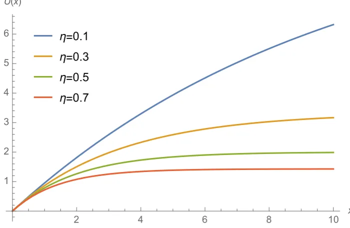
Figure 2.1: Comparison of Weibull Distributions with Different Shape Parameters

η: Probability Density Functions left), Cumulative Distribution Functions

(top-right), Survival Functions (bottom-left), Hazard Functions (bottom-right).

When the scale parameter α = 1, Figure 2.1 shows a number of Weibull

proba-bility density functions, cumulative distribution functions and corresponding hazard

functions, respectively.

The mean and variance of the Weibull can be expressed in terms of the gamma

function which is defined below.

Definition 2.12 Gamma Function For a > 0 the gamma function is defined to be

Γ(a) =

Z ∞

0

xa−1e−xdx.

The next theorem gives the mean and variance of the Weibull distribution in terms of

the gamma function.

Proposition 2.1 If X ∼W EI(η, α), then

E(X) = αΓ

1 + 1 η

(36)

and

V(X) = α2

"

Γ

1 + 2 η − Γ

1 + 1 η

2#

(2.10)

See Rigdon and Basu (2000) for proofs.

Gamma Distribution

The gamma distribution is another useful model for the lifetime of systems.

Definition 2.13 The pdf for the gamma distribution can be written as

f(x) = x

η−1

θη_Γ(η)exp(−x/θ), x >0.

We will write X ∼ GAM(η, θ) if the random variable X has this pdf, where η and θ

are the shape and scale parameters, respectively. Another useful form for the gamma

pdf is obtained by substituting 1/λ for θ; this gives

f(x) = λ

η_xη−1

Γ(η) exp(−λx), x >0. (2.11)

The cdf and the survival function, and hence also the hazard function, cannot be

written in closed form. We can write the cdf as

F(x) =

Z x

0

ληωη−1

Γ(η) exp(−λω)dω.

If we make the transformation y=λω, then this becomes

F(x) =

Z λx

0

λη_(y/λ)η−1

Γ(η) e

−y1

λdy

= λ

η

λη−1_Γ(η)

1 λ

Z λx

0

yη−1e−ydy

= 1

Γ(η)

Z λx

0

yη−1e−ydy.

The hazard function is therefore

h(x) = f(x)

1−F(x)

=

λη_xη−1

Γ(η) exp(−λx)

1− 1 Γ(η)

Rλx

0 y

η−1_e−y_dy.

This hazard function is increasing when η > 1, decreasing when η < 1, and constant

(37)

η=1.8

η=1

η=0.6

1 2 3 4 5 x

0.2 0.4 0.6 0.8 PDF

η=1.8

η=1

η=0.6

1 2 3 4 5 x

0.2 0.4 0.6 0.8 1.0 CDF

η=1.8

η=1

η=0.6

1 2 3 4 5 x

0.2 0.4 0.6 0.8 1.0 Survival

η=1.8

η=1

η=0.6

1 2 3 4 5 x

[image:37.595.99.539.53.347.2]

0.5 1.0 1.5 Hazard

Figure 2.2: Comparison of Gamma Distributions with Different Shape Parameters

η: Probability Density Functions left), Cumulative Distribution Functions

(top-right), Survival Functions (bottom-left), Hazard Functions (bottom-right).

When the scale parameter θ = 1, Figure 2.2 shows a number of gamma

proba-bility density functions, cumulative distribution functions and corresponding hazard

functions, respectively.

2.2

Maintenance Modelling

Traditional repairable systems assume a whole range of performance levels, varying

from perfect functioning to complete failure, and assuming the repair is perfect.

How-ever, many manufacturing systems suffer increasing wear with usage, age or

deteri-oration, that is, perfect functioning is not always satisfied. Therefore, maintenance

management, as an important policy for a repairable system, is widely used to keep

systems in good condition, to decrease failures, and increase system availability. Based

on the European standard (EN 13306:2010), a definition of maintenance management

(38)

Definition 2.14 Maintenance Management depicts all activities of the manag-ment that determine the maintenance objectives, strategies and responsibilities, and

implementation of them by such means as maintenance planning, maintenance control,

and the improvement of maintenance activities and economics.

According to the definition above, the major steps to maintenance modelling can

be summarised as:

1. Determine the maintenance objective(s).

2. Define or select maintenance policies according to measures of system

perfor-mance.

3. Plan, control and improve maintenance.

2.2.1

Maintenance Policies

The availability and usability play a crucial part in a system’s performance because

any breakdowns and holdups can seriously impede its performance. At the same time,

idle systems negatively affect the ratio between fixed cost to output. The reduced

output induced by system breakdowns would result in less production as well as less

profitability which can be regarded as an inefficiency for the system. Moreover, complex

systems usually require a significant startup time after an interruption occurs. Possibly

during this period of time, goods that do not meet acceptable levels,e.g., scrap or goods

of minor quality are produced, as a result, one cannot obtain her or his expected profit

since these products cannot be sold or have to be sold at reduced prices. Thus, efficient

operation of a system requires well-scheduled maintenance to avoid interruptions as

much as possible and to recover from breakdowns quickly.

For a manufacturing system, wear-out, ageing and deteriorating will have a negative

impact on the function of the system, which results in the consequence that the system

cannot fulfil its capability. Maintenance is introduced to counteract those negative

ef-fects from an economic point of view. Therefore, maintenance actions plays an essential

role in sustaining and possibly improving a system’s availability, which in return will

improve the productivity of the system considered. In general, maintenance policies

and strategies are commonly categorised into three domains: Corrective Maintenance

(39)

Corrective maintenance is initiated when the system sees a breakdown which results

in a stop for a system working and induces considerable cost. Corrective maintenance

is usually named repair, restoration or replacement of failed components. This

mainte-nance policy is often applied to systems of which failure is not costly and do not result

in disastrous situations, for components with constant failure rate,e.g., if a failure time

of components is assumed to follow an exponential distribution.

Preventive maintenance is implemented for the purpose of minimising the

nega-tive impact of an unexpected breakdown. Generally speaking, prevennega-tive maintenance

usually involves less resource consumption compared to that of corrective maintenance

and it can be designed in the production plans of the system of interest. PM

in-cludes all partial or complete overhauls, such as filter cleaning, oil charging, etc. in

order to prevent a critical failure that is costly before it actually occurs. It can be

seen that preventive maintenance makes sense in the situation when the failure rate

of a unit or component is increasing in time. Unlike CM that is unexpected,

preven-tive maintenance can usually be properly planned and prepared. Although prevenpreven-tive

maintenance is incorporated to prevent critical failures in system designing, sometimes

failure may still be seen. As a result, it is usually suggested to combine both corrective

maintenance and preventive maintenance tasks.

However, when the operation schedules and environmental variables change in

prac-tice, exhaustive or unnecessary use of preventive maintenance can occur. To make

sure that preventive maintenance is taken only when it is required, condition based

maintenance was introduced by incorporating inspections of the system of interest in

pre-determined intervals to determine the system’s operation condition. Depending on

the outcome of an inspection, relevant maintenance tasks can be implemented. It is

worthwhile noting that CBM is sometimes analysed in the field of PM (Manziniet al.,

2010).

The preventive maintenance policies include time based PM (Roux et al., 2008) in

which PM is conducted every t units of time and age based PM (Chen et al., 2006)

where PM is carried out every t units of operating time. There are other alternatives

of preventive maintenance, e.g., for non-repairable systems, group block replacements

where units or components would be replaced if it failed whereas the other working

(40)

Condition based maintenance has received less attention probably because it is

rel-atively new compared to CM and PM. However, thanks to the fact that the inspection

is less costly, one is encouraged to implement CBM (Xiang et al., 2012). If a system

is designed to serve for a long period, one inspection monitor can be installed if it is

relatively cheaper. Van Horenbeek and Pintelon (2013) proposed a prognostic

mainte-nance by combining CBM with the prediction about the states of components to see

if a threshold is expected to be reached before the following scheduled inspection. If it

does, the component is replaced immediately. Although it can be seen that there is an

increasing application of CBM in practice (Wang et al., 2008), it is less studied in the

literature.

In reviewing the literature, we find limited effort was taken to compare

differ-ent maintenance policies. Xiang et al. (2012) investigated a repairable system

un-der preventive maintenance and condition based maintenance policies and found that

condition-based maintenance is superior to scheduled maintenance paradigm via

simu-lation. Van Horenbeek and Pintelon (2013) studied five different maintenance policies

(i.e., CM, block PM, age based PM, CBM with inspection and CBM under continuous

monitoring) on one machine and their noted effects.

2.2.2

Maintenance Effectiveness

Preventive maintenance comprises all maintenance activities which are not triggered

by a system failure. Not only the mode of maintenance task (preventive maintenance

or corrective maintenance) and its associated maintenance interval impact the failure

rate, but also its level of quality (effectiveness of maintenance task). The state after a

maintenance action is performed on a component is assumed to be: perfect, imperfect,

(41)

Maintenance Policy System State Failure Rate

Preventive maintenance The system state is

re-stored to be “as good

as new”

Decreasing of the failure rate

Imperfect maintenance A maintenance action

that restores the

system to a state

somewhere between

“as good as new” and

“as bad as old”

Decreasing of the failure rate

Minimal Maintenance The system state is

“as bad as old”

No effect on the failure rate

Worse Maintenance System is in

operat-ing state worse than

just prior to the

main-tenance action

Increasing of the failure rate

Worst maintenance System breaks down

right after

mainte-nance action

Increasing of the failure rate

Table 2.1: State assumptions after maintenance

Imperfect, worse or worst maintenance can be caused by repairing parts of a system

mistakenly. In addition to one of the best known models proposed by Brown and

Proschan (1983), Pham and Wang (2006) reviewed other approaches to model imperfect

maintenance, such as (p, q) rule, (p(t), q(t)) rule, improvement factor, and virtual age

approach, etc. Briefly, with probability p, the item is restored to the as good as new

state or otherwise to the as bad as old state with probability q = 1− p. A novel

approach to modelling imperfect preventive mainteannce will be propsed in Chapter 5.

Quality levels of worse and worst maintenance are related to maintenance and repair

induced failures. Preventive maintenance actions, as cleaning or greasing, mitigate the

deterioration effect of some failure mechanics and restore components to a “as good

(42)

mechanisms will remain unaffected. Hence, Lin et al. (2001) introduced the concept

of two categories of failure mechanisms, maintainable failure mechanisms and

non-maintainable failure mechanisms. Preventive maintenance will affect maintainable

fail-ure mechanisms exclusively, whereas non-maintainable mechanisms remain unaltered.

Zequeira and Berenguer (2005) stated that the maintainable and non-maintainable

failure rates are dependent and restored the system of interest to a condition between

as good as new and as bad as old via their proposed preventive maintenance actions.

In the literature, three approaches for modelling the impact of preventive

mainte-nance on the failure rate have been studied extensively; a failure rate model by Lie

and Chun (1986) and Nakagawa (1986), Nakagawa (1988), an age reduction model by

Canfield (1986) and Malik (1979) and a hybrid model by Lin et al. (2001).

In maintenance modelling, most researchers model a system as a whole unit,

with-out considering the effect of deterioration and failure on the subsystems. On the other

hand, machines were modelled as subsystems by some researchers. Van Horenbeek

and Pintelon (2013) modelled a simplified version only considering one subsystem in

a few machines and analysed the structural and stochastic dependencies. Roux et al.

(2008) evaluated the impact of three maintenance policies under an assumption that a

system has only two independent components. One of the assumptions in maintenance

modelling is assuming all the units or components of a system are identical and

inde-pendent. There are other less rigorous assumptions and we will include some of them

in our research:

• Perfect maintenance: preventive maintenance is assumed to be done perfectly

and it is often referred to as ‘systems are are good as new’ after preventive

maintenance is conducted. In this thesis, perfect preventive maintenance (PPM)

is equivalent to corrective maintenance (CM) in the sense that they have the

same consequence with regard to the state of the system after maintenance.

• Time of implementing maintenance is assumed to be constant and often is even

reduced to be negligible implying that maintenance is carried out instantaneously.

• Costs of all relevant maintenance tasks are assumed to be known as constant and

the cost of CM is always more than that of PM.

(43)

conduct maintenance.

• System failures are assumed to be detected immediately.

2.2.3

Sequential Maintenance

Under sequential maintenance, systems may be maintained at unequal time intervals,

in contrast to periodic maintenance in which the maintenance interval is fixed and

unique.

Barlow and Proshan (1965) design a sequential maintenance policy for a finite time

span. Under this maintenance policy, the time for which maintenance is scheduled

depends on the time remaining rather than the pre-determined and identical

mainte-nance time. In addition, the next maintemainte-nance interval is determined by minimising

the average cost per unit time during the remaining time. Therefore, this policy does

not determine systems’ future maintenance intervals at the initial time of system

per-formance, which adds flexibility and reduces systems costs.

Nguyen and Murthy (1981) model preventive maintenance under a sequential policy

in which a failure needed to be corrected has not occurred by a reference timeti, whereti

is the maximum time that a system should be fully replaced without extra maintenance

after the (i−1)th _{repair; in other words, the system is replaced after (k}₋_{1) repairs.}

The system is repaired (or replaced at the kth repair) at the time of failure or at time ti, whichever occurs first.

Nakagawa (1986) propose and compare periodic and sequential preventive

nance policies for the system with minimal repair at failure and compute the

mainte-nance intervals in a Weibull distribution case, indicating that a sequential preventive

maintenance policy is superior to a periodic one. Schutzet al. (2011) extend previous

research by considering a system performing a wide range of missions over a finite

plan-ning horizon and a dynamic system failure law is taken into account to modelling the

different missions with various characteristics depending on the operational conditions.

Linet al. (2000) propose general sequential imperfect preventive maintenance models,

in which the effective remaining time of the system would be reduced whilst the hazard

rate would be adjusted after each preventive maintenance. We refer it to as a hybrid

(44)

hazard adjustment on systems.

There are also studies by Dieulle et al. (2003) calculating the long-time expected

cost per unit of time via considering if system’s state is above or below a threshold and

assuming deterioration as a gamma process; and Schutzet al. (2011) investigating the

periodic and sequential preventive maintenance policies over a finite planning horizon.

However, due to the highly mathematical formalisation of their modelling, it is not

staightforward to be applied in practice.

2.3

Maintenance Optimisation

2.3.1

Optimisation Approaches

As the complexity of maintenance systems increases, maintenance optimisation

meth-ods have also developed from classical methmeth-ods to modern or non-traditional methmeth-ods.

Classical optimisation methods (Rao, 2009) are analytical and use differential

cal-culus to find the optimal value. For example, scatter search (Chenet al., 2006),

Nelder-Mead method (Roux et al., 2008, 2013), cyclic coordinate method (Xiang et al., 2012),

the modified Powell method (Marquez et al., 2003), Fibonacci algorithms (Asadzadeh

and Azadeh, 2014) and local search (Gupta and Lawsirirat, 2006; Triki et al., 2013),

have been applied to simple manufacturing systems. However, it has been criticised

that optimising maintenance through classical methods lacks the analysis of objective

functions and solution space. Thus it poses difficulty in justification of the optimisation

methods.

In order to deal with the complexity increase of maintenance systems, modern

or non-traditional methods have been utilised (Deb, 2005; Rao, 2009). Two modern

optimisation methods are mainly applied, which are Genetic Algorithms (GA) and

Simulated Annealing (SA). In fact the use of SA is only reported in a few articles. In

this sense, exploration of other modern optimisation methods to systems maintenance

problems could be another research branch.

The most reported modern optimisation method in maintenance, GA, is based upon

the process of natural selection in biology and has been applied to various optimisation

problems (Rao, 2009). SA originates from the idea of the annealing process in

(45)

beginning and then cooled gradually under a fully controlled environment to obtain

desirable shapes or properties. This method has been used to solve a wide variety of

problems, such as the ones with continuous, discrete and mixed-integer variables (Rao,

2009).

Dynamic programming (DP), see Bellman (1954), is a method of solving a

com-plex problem by breaking it down into series of simpler subproblems (different parts

of the original problem) and then combining the solutions to the subproblems to

ob-tain an overall solution to the original problem. There are two advantages using this

formulation. First, dynamic programming enables computing the optimal solution in

some cases which usually only applies to smaller problems. Due to the curse of

di-mensionality, computing the optimal solution to larger problems cannot be done in

a reasonable and feasible amount of time (Powell, 2007). Second, dynamic

program-ming can produce optimal theoretical results which could indicate the behaviour of the

optimal policy in the proposed models, for example, see Ding et al. (2002).

In a general assumption about state, action and parameter spaces, Rieder (1975)

consider a non-stationary Bayesian dynamic decision model which can be reduced to

a non-Markovian decision model with known transition probabilities. As a

pioneer-ing work in Bayesian dynamic programmpioneer-ing, his work provides criteria of optimality

and the existence of Bayes policies. Nicolato and Runggaldier (1999) combine

burn-in, which is used to cope with the problem of “infant mortality” in system running

periods, with identical multi-component systems, and propose a Bayesian dynamic

programming method to make decisions on the optimal maintenance interval and best

burn-in time.

In other words, dynamic programming is an optimisation approach that transforms

a complex problem into a sequence of simpler problems; its essential characteristic is the

multistage nature of the optimisation procedure, which provides a general framework

employed to solve particular aspects of a more general formulation. In the decision

tree problem, we often call it “Roll-Back”, see Ross (1995). As in the problem we

will discuss in the next chapter, we divide the system’s running procedure into a few

stages and based on the information we learn from running the system, we model the

functional form of the system utility and then attempt to maximise it.

(46)

problem. We consider the system running from a global perspective, which means we

assume the whole running procedure of the system, and make a decision based on the

optimal utility of the system. On the contrary, myopic decision making means that

we can do local utility optimisation based on the information we previously obtained.

Although we would not obtain the optimal utility for the system, optimisation problems

can be simplified and are also easier to implement in practice, and we can simply regard

it as a “roll-forward” method.

2.3.2

Optimisation Objectives

Cost minimisation is one of the most reported optimisation objectives in maintenance

studies, for example, minimising total cost or expected cost per unit time. Increasing

preventive maintenance cost could result in over-maintenance for systems while

increas-ing hazard rate and its consequences would end up with under-maintenance. Note that

usually corrective maintenance cost is fixed and higher than preventive maintenance

cost (Gupta and Lawsirirat, 2006; Rouxet al., 2008; Xianget al., 2012). However, it is

not sufficient to simply only consider maintenance cost as maintenance is part of

sys-tems and various costs are associated with syssys-tems processing. Thus some researchers

have incorporated other costs, in addition to maintenance cost, into maintenance

ob-jectives. For instance, a penalty per unit time for systems unavailability (Alrabghi and

Tiwari, 2013), or the cost resulting from unsatisfactory products (Oyarbide-Zubillaga

et al., 2008).

On the contrast to maintenance cost, Roux et al. (2013) propose maximising

sys-tems availability as the optimisation objective. They argue that it is more justified as

production costs are more dominant in the total cost of systems running. However,

such interpretation would ignore the fact that maintenance costs can be higher than

production costs (Wang et al., 2008).

However, it is suggested to design the objective as maximising production

through-put because maximum system availability does not necessarily guarantee maximum

production throughput (Lei et al., 2010) because a system would not be in a working

state due to various reasons such as lack of raw materials or supporting tools.

On the requirements of different engineering problems, optimising several

(47)

average cost per unit time and maximising systems availability. There are mainly

three ways to realise this aim: firstly, put several objectives into one objective

func-tion, however, this method requires transformation in a universal unit among different

objectives; secondly, assign weights to different objectives based on decision maker’s

preference. Although transformation is not required in this method, the decision maker

has to trade-off among objectives; thirdly, simply solve several objectives

simultane-ously using multi-objective optimisation algorithms, e.g., Oyarbide-Zubillaga et al.

(2008) implement a Non-dominated Sorting Genetic Algorithm to minimise costs as

well as maximise system production profits.

The objective proposed in this thesis is utility-based maintenance. From the

main-tenance engineer’s point of view, by incorporating risk preferences into mainmain-tenance

modelling, management of systems could avoid short-term problems such as short-term

cash flow problems by considering optimal long-term policy such as systems

availabil-ity. For example, there are two policies that are equally preferred based on minimising

average cost per unit time, however, it is likely that one of them has more variable

(48)

(49)

Chapter 3

Statistical Methodology and Utility

In operational research and management science we face uncertainty frequently, whether

in the form of uncertain demand for production, uncertain performing time in systems,

or uncertainty about parameters calibrating a simulation model,etc. Despite the fact

that we are facing uncertainty, we usually are able to collect some related information

which could reduce the effects of such uncertainty. This would have two impacts: on

one hand, gathering information helps us make better decisions which could produce

better outcomes; on the other hand, the costs induced by collecting information, such

as time and money spent, or even opportunity cost due to collecting one piece of

infor-mation whereas we could have had another, could increase. How to find the optimal

balance between these benefits and costs is what we are attempting to explore. Two

methods for formulating such problems are Bayesian methods and Dynamic

Program-ming, respectively.

3.1

Bayesian Modelling

In the twentieth century, the so called ‘frequentism’ has dominated the statistical

phi-losophy. Under the framework of the frequentist approach, the hypothetical long term

proportion of the time that an event of interest occurs is expressed via probability and

the parameters of probability models are regarded to be unknown but fixed

numeri-cal quantities. Pearson studied the problems of the frequentist style extensively in the

early twentieth century. One can find most of the foundations for frequentist modelling

(50)

Bayesian modelling arises earlier than the frequentist methodology actually. It is

being dated back to a thought experiment conducted by Bayes (1763) who threw balls

onto a square table, and to the ‘inverse probability’ found by Laplace (1774) and later

replaced as ‘Bayesian’ in the 1950s by Fisher (Fienberg, 2006). Both Bayes and Fisher

took the uniform prior distribution: it was a outcome of the ball throwing experiment

in Bayes’ case, while it was considered as an intuitive axiom which is a ‘principle of

insufficient reason’ by Fisher. Yet, Bayesian modelling and inference has not drawn

much attention until it reappeared and was recognised in the modern form thanks to

Jeffreys (1939) and Savage (1954), among other researchers.

Briefly the Bayesian concept combines both objective probability that has a similar

interpretation compared to the probabilities in frequentism and subjective probability

that is taken to express a degree of belief from a personalistic point of view. The

treatment of regarding the parameters of probability models as realisations of a random

variable or not differentiate Bayesian modelling from frequentist methodology, and

enable one to put direct statements of probability for these parameters.

Let us consider a sequence of observations x = {x1, . . . , xn} and a corresponding

probability model that is believed to be the generating model for the data, with a

probability density function fX(x|ψ) in which the parameter(s) ψ is made explicitly

to model the dependence. It is worthwhile noting thatψ may be a vector of parameter

in general. ψ is considered as the unknown realisation of a random variable in the

Bayesian modelling, as a result we can consider the joint density function of the random

variables X and Ψ:

fX,Ψ(x, ψ) =fX|Ψ(x|ψ)fΨ(ψ) (3.1)

where fX|Ψ(x|ψ) :=fX(x|ψ) for simplicity.

As a result, given data x, one can apply Bayes’ Theorem to directly derive the

uncertainty expression for ψ as:

fΨ|X(ψ|x) =

fX(x;ψ)fΨ(ψ)

R

ΩfX(x;ψ)fΨdψ

(3.2)

∝fX(x;ψ)fΨ(ψ)

where Ω is the sample space of Ψ. Notice that the denominator is independent of ψ

(51)

(3.2) is referred to as the posterior distribution of parameter(s) ψ and encapsulates all

knowledge and information concerning the unknown parameters.

However, in practice the integral in the denominator of (3.2) which is the

normal-ising constant, does not often have an analytically tractable form. Due to this fact,

it hindered the learning and application of Bayesian modelling for quite a long period

of time. With the rapid development of computing techniques such as Markov chain

Monte Carlo in modern time, Bayesian modelling has become easier to implement since

the 1990s.

3.1.1

Likelihood function

In (3.2), the first term in the numerator is usually written as L(ψ;x) := fX(x|ψ) to

indicate the fact that the observed data xare fixed and ψ is in fact stochastic. Fisher

(1922) terms this the likelihood, arguing that it was all necessary to do inference

through simply maximisingL(ψ;x) with regard toψ and one can obtain the maximum

likelihood estimate (MLE), ˆψ. However, due to the fact that R_ΩL(ψ;x)dψ 6= 1, we can not take the likelihood as a probability distribution function for ψ, which makes

expressing the uncertainty about the point estimate ˆψ somewhat more ambiguous than

the expression in the form of posterior distribution in Bayesian modelling.

In favour of the ‘fiducial probability’ of ψ, Fisher (1930) defined _∂ψ∂ FX(x;ψ) as a

way to connect ψ to a direct probability uncertainty. However, after extensive

criti-cism, e.g.(Lindley, 1958), almost nobody refers to this idea in the modern literature.

Therefore, based on asymptotic analysis, the expression of uncertainty for ˆψ is limited

to be required to state the upper/lower confidence bound for non-standard models,

which is argued to contain the ‘true’ ψ in terms of a specified hypothetical long run

proportion.

Still only in the way of the likelihood can the data enter the posterior distribution

to be utilised. And as the amount of data collected increases, the likelihood part

dominates the posterior distribution more, resulting in approximate agreement between

maximum likelihood estimate for frequentists and highest a posteriori density values

for Bayesians, which is the mode of the posterior distribution. In Bayesian modelling,

any two models with the same likelihood L(ψ;x) are believed to result in the same

(52)

called the ‘likelihood principle’.

3.1.2

Prior distribution

The prior distribution is the termfΨ(ψ) in numerator from (3.2). Because the

param-eters are treated as random variables in Bayesian modelling, a Bayesian is required to

specify corresponding distributions for the random variables which are independent of

the dataxin (3.1). The prior distribution is taken to represent the information that a

decision maker has known prior to observing any possible data and is usually regarded

as the most controversial part in Bayesian methodology.

The controversy arises owing to the fact that the choice of a prior distribution

is always a subjective decision. However, it is argued that the implementation of a

prior distribution adds flexibility of modelling. For example, we can choose a ‘sceptical

prior’ which is suggested to assign a lower probability to some favourable outcomes.

Thus, the probability weighs in favour of that outcome becomes even more compelling.

However, we can think that the chosen model that is believed to be where the data are

generated, fX(·;ψ) is also a somewhat subjective choice.

Common prior choices

In Bayesian modelling and inference, the prior is often chosen from some parametric

family o

Bayesian modelling and analysis of utility based maintenance for repairable systems

Bayesian Modelling and Analysis of

Abstract

Acknowledgements

Abbreviations

Contents

List of Tables

List of Figures

Chapter 1

Structure and Main Contributions

Chapter 2

Reliability Measures

Classical Failure Distributions

Maintenance Modelling

Maintenance Policies

Maintenance Effectiveness

Sequential Maintenance

Maintenance Optimisation

Optimisation Objectives

Chapter 3

Bayesian Modelling

Likelihood function

Prior distribution