Original citation:
Sonnenwald, Fred, Stovin, Virginia and Guymer, Ian. (2014) Configuring maximum entropy deconvolution for the identification of residence time distributions in solute transport applications. Journal of Hydrologic Engineering, Volume 19 (Number 7). pp. 1413-1421.
Permanent WRAP url:
http://wrap.warwick.ac.uk/65102
Copyright and reuse:
The Warwick Research Archive Portal (WRAP) makes this work by researchers of the University of Warwick available open access under the following conditions. Copyright © and all moral rights to the version of the paper presented here belong to the individual author(s) and/or other copyright owners. To the extent reasonable and practicable the material made available in WRAP has been checked for eligibility before being made available.
Copies of full items can be used for personal research or study, educational, or not-for profit purposes without prior permission or charge. Provided that the authors, title and full bibliographic details are credited, a hyperlink and/or URL is given for the original metadata page and the content is not changed in any way.
Publisher’s statement:
Link to published version: http://ascelibrary.org/doi/10.1061/%28ASCE%29HE.1943-5584.0000929
A note on versions:
Configuring maximum entropy deconvolution for the identification
1
of residence time distributions in solute transport applications
2
F. Sonnenwald1, V. Stovin2, I. Guymer3
3
ABSTRACT 4
The advection-dispersion equation (ADE) or aggregated dead zone (ADZ) models and
5
their derivatives are frequently used to describe mixing processes within rivers, channels,
6
pipes, and urban drainage structures. The residence time distribution (RTD) provides a
7
non-parametric model that may describe mixing effects in complex mixing contexts more
8
completely. Identifying an RTD from laboratory data requires deconvolution. Previous
9
studies have successfully applied maximum entropy deconvolution to solute transport data,
10
with RTD sub-sampling used for computational simplification. However, this requires a
11
number of configuration settings which have to date not been rigorously investigated. Four
12
settings are investigated here: the number and distribution of sample points, the constraint
13
function, and the maximum number of iterations. Configuration options for each setting
14
have been systematically assessed with reference to representative solute transport data
15
by comparing the goodness-of-fit of recorded and predicted downstream profiles using the
16
Nash-Sutcliffe Efficiency Index, evaluating RTD smoothness with a measure of entropy, and
17
through consideration of the mass-balance of the RTD. New methods for defining sample
18
point distribution are proposed. The results indicate that goodness-of-fit is most sensitive to
19
constraint function and that smoothness is most sensitive to the number and distribution of
20
sample points. A set of configuration options that includes a new sample point distribution
21
1PhD Student, Department of Civil & Structural Engineering, The University of Sheffield, Mappin St.,
Sheffield S1 3JD, UK, e-mail: [email protected]
2Senior Lecturer, Department of Civil & Structural Engineering, The University of Sheffield, Mappin St.,
Sheffield S1 3JD, UK, e-mail: [email protected]
3Professor, School of Engineering, University of Warwick, Coventry CV4 7AL, UK, e-mail:
is shown to perform robustly for a representative range of laboratory solute transport data.
22
Keywords: Solutes, Dispersion, Mixing, Hydraulic models, Transfer functions
23
INTRODUCTION 24
Background
25
Solute transport is affected by mixing processes. As such, improved understanding of
26
solute transport can lead to both new applications in water quality modelling and to improved
27
understanding of the underlying processes that affect mixing. This applies to processes in
28
natural rivers and channels as well as man-made structures such as pipes and manholes.
29
The advection-dispersion equation (ADE) or aggregated dead zone (ADZ) models have
30
traditionally been used to evaluate or model solute transport (Rutherford 1994). Both are
31
parametric models that apply an understanding of the processes involved to derive a system
32
of equations. They include assumptions and, provided they are met, the models can perform
33
extremely well, e.g. in pipe flow (Taylor 1954). Model performance degrades when the
34
underlying assumptions are not met (Davis et al. 2000; Rieckermann et al. 2005).
35
In chemical engineering, the residence time distribution (RTD) is frequently used to
36
describe mixing within reactors in response to a Dirac pulse (an instantaneous input)
(Lev-37
enspiel 1972). Equation 1 shows the relationship between upstream y(t) and downstream
38
u(t) temporal concentration data through convolution with the RTD h(t). The RTD is also
39
known as a transfer function. In hydrology the RTD is analogous to the unit hydrograph
40
(Sherman 1932).
41
y(t) =
Z ∞
−∞
h(τ)u(t−τ)dτ (1)
42
Recent research has used the RTD to describe solute transport in urban drainage systems,
43
e.g. Guymer and Stovin (2011). The particular benefit of an RTD is that, as a
non-44
parametric model, no assumptions are made on how the system operates. Therefore, the
45
RTD can exactly describe complex mixing processes in a reach or structure, such as dead-zone
short-circuiting (Stovin et al. 2010a). Unfortunately this benefit incurs a cost, as identifying
47
an RTD is significantly more complex than identifying the parameters of traditional models.
48
The general method of identifying an RTD from recorded laboratory data is
deconvo-49
lution. There are many methods and applications for deconvolution. An overview of some
50
common methods is given by Madden et al. (1996). Other applications include noise
cancel-51
lation (Pandolfi 2010) and gas chromatography (Zhong et al. 2011). Within solute transport
52
research, deconvolution techniques have been used to examine soil transfer functions (Skaggs
53
et al. 1998), bank filtration (Cirpka et al. 2007), and transient storage (Gooseff et al. 2011).
54
We have previously used maximum entropy deconvolution to investigate solute transport in
55
manholes (Stovin et al. 2010b; Sonnenwald et al. 2011; Guymer and Stovin 2011).
56
Although maximum entropy deconvolution has previously been successfully applied to
57
solute transport data, no rigorous investigation into how the configuration settings affect
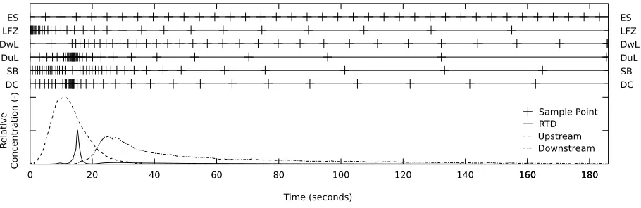
58
the quality of the results obtained has been reported. Four maximum entropy deconvolution
59
settings impact on the quality of the deconvolved RTD: the number of sample points; sample
60
point distribution; constraint function; and the maximum number of iterations.
Inappro-61
priate configuration options for any of the settings may result in a poor quality RTD. This
62
paper aims to systematically identify a robust set of options that can be used to deconvolve
63
the RTD from typical solute transport data. To this end, a sensitivity analysis has been
64
carried out with a range of data and options.
65
Maximum entropy deconvolution
66
Maximum entropy deconvolution is a discrete computational technique that uses regularly
67
sampled paired upstream and downstream temporal concentration profiles to deconvolve the
68
RTD. An estimate of the RTD, ˆh = {h1, . . . , hN} where N is the number of data points, 69
is to be made as flat as possible with the only exceptions being those implied by the
up-70
stream and downstream data (Skilling and Bryan 1984). Flatness of ˆh is measured by an
71
entropy functionS, Equation 2, which also enforces non-negativity. A constraint functionC,
72
Equation 3, ensures that the RTD is valid by comparing the goodness-of-fit of the predicted
downstream concentration profile ˆy against the recorded profile y, where ˆy is calculated as
74
the convolution of ˆhandu. C is typically, as presented here, the chi-squared function, where
75
σ is an error estimate. The RTD is identified by combining both equations in a Lagrangian
76
function L, Equation 4, and maximizing. λ is the Lagrange multiplier determined during
77
the maximization process. Sub-scripts denote specific points in discrete time.
78
S(ˆh) = − N X
i=1
ˆ hi PN
j=1ˆhj
ln
ˆ hi PN
j=1ˆhj
(2)
79
C =
N X
i=1
(ˆyi−yi)2/σi2 (3) 80
L(ˆh, λ) = S(ˆh)−λC (4)
81
The software and methodology used for maximum entropy deconvolution of solute
trans-82
port data is an evolution of a pharmacokinetics application (Hattersley et al. 2008). In
83
pharmacokinetics, data points are often collected at uneven time intervals, e.g. by a nurse
84
making rounds. As a result, the entropy function was modified for piecewise data, where
85
the value between points is assumed to vary linearly, and Equation 5 was developed. The
86
r term is added as a base-line prediction of the RTD in the absence of other data. r takes
87
the form of a nearest neighbour moving average where ri = ((ˆhi−1 + ˆhi+1)/2) and at i = 0
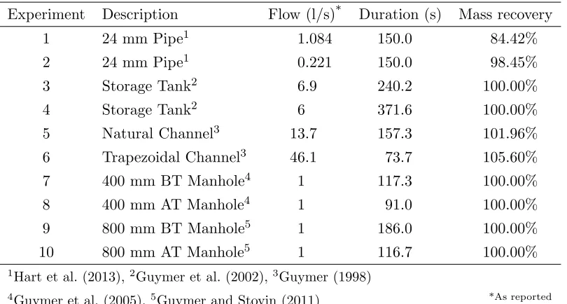
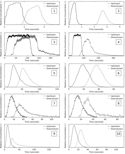
88
and i=N the value of the two nearest points, e.g. rN = (ˆhN−1+ ˆhN)/2. The inclusion of r 89
results in an entropy value that evaluates smoothness; entropy values closer to zero indicate
90
a smoother function.
91
S(ˆh) = − N X
i=1
ˆ hi PN
j=1ˆhj
ln
ˆ
hi/PNj=1ˆhj
ri
(5)
92
To obtain ˆh, Hattersley et al. (2008) converted Equation 4 into an equivalent minimisation
93
problem. This was solved using a Sequential Quadratic Programming (SQP) technique
implemented in Matlab, fmincon (The MathWorks Inc. 2011). SQP is an optimisation
95
algorithm that works by minimising a quadratic model of the problem to find the next step
96
towards the solution (The Morgridge Institute for Research 2012).
97
Maximum entropy deconvolution was further modified for application to solute transport
98
data by Stovin et al. (2010b). The piecewise capability previously introduced was modified
99
to create a simplified deconvolution problem where the RTD is sub-sampled. This reduces
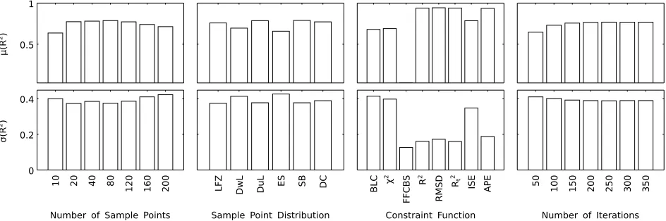
100
computational expense and the impact of noisy data while maintaining the benefits of a
101
non-parametric model. The sub-sampled RTD is defined only at n sample points, spread
102
between the start and end of the concentration data, as the length of the RTD is unknown.
103
Sample points are otherwise placed where more variation is expected in the RTD. A full
104
RTD is reconstructed from the sub-sampled RTD using linear interpolation.
105
METHODOLOGY 106
Configuration settings for maximum entropy deconvolution
107
The first two configuration settings are number and positioning of sample points. As
108
linear interpolation is used to reconstruct the RTD, each sample point defines a change in
109
the slope of the RTD. Therefore, changing the position and number of points is expected to
110
have a high impact on the identified RTD.
111
Skilling and Bryan (1984) suggest that alternative constraint functions may be
prefer-112
able to χ2, hence this configuration setting is also examined here. AsC effectively evaluates
113
goodness-of-fit, correlation measures form suitable alternatives. Different correlation
mea-114
sures may place different emphasis on matching the shape, scale, or noise (Sonnenwald et al.
115
2013).
116
fmincon introduces the fourth configuration setting, maximum number of iterations,
117
which imposes an upper limit on fmincon so that it does not enter an infinite loop. Too
118
few iterations, however, will stop the deconvolution process before convergence is achieved,
119
i.e. before the RTD is identified. fminconalso introduces convergence criteria to determine
when optimisation stops and an ‘initial guess’ that is the start point of the optimisation
121
process.
122
Number of sample points 123
Stovin et al. (2007) suggested that as few as 7 points are necessary to define an RTD. A
124
minimum of 10 sample points has therefore been used. 20, 40, 80, 120, 160, and 200 sample
125
points have also been evaluated. After 200 points we have observed computational cost to
126
increase significantly. Stovin et al. (2010b) used 40 sample points.
127
Sample point distributions 128
Sample points are placed where more variation in the RTD is anticipated by incorporating
129
basic assumptions of the expected RTD. Six sample point distributions have been developed
130
using varying amounts of prior knowledge, described below and shown in Figure 1.
131
• Equally spaced (ES): The sample points are evenly distributed across the input
132
data. This distribution assumes no knowledge of the RTD.
133
• Log from zero (LFZ):The interval between sample points increases logarithmically
134
from the start to the end of the data. This distribution assumes more variation earlier
135
in the RTD and less variation as time goes on, i.e. an exponential decay.
136
• Downstream log (DwL): First arrival time and end of event are defined as 1% of
137
peak concentration. Three sample points are evenly distributed from the start of the
138
data until the difference in first arrival times, after which the interval between sample
139
points increases logarithmically until the end of the downstream event. Three more
140
sample points are evenly distributed until the end of data. From Equation 1 it follows
141
that there must be some delay in the RTD if there is a delay between first arrival
142
times. This is the sample point distribution previously used by Stovin et al. (2010b).
143
• Double log (DuL): Half of the sample points are distributed logarithmically from
144
the start of the data to the difference in time to peak, which is used as an estimate
145
of delay. The other half of the sample points are logarithmically distributed away
from the difference in time to peak to the end of the data. A greater concentration
147
of points around the time the RTD peak is expected allows for more uncertainty in
148
its location.
149
• Slope based (SB): This is a new development. An approximation of the RTD
150
is used to distribute the sample points where slope is expected to be greater. The
151
approximation is computed using Fast Fourier Transformation (FFT) deconvolution
152
(Madden et al. 1996) with Blackman-Tukey Windowing (Blackman and Tukey 1958;
153
Harris 1978) applied to the input data to improve accuracy. The absolute area of the
154
first derivative of the approximation is evenly divided and sample points placed at
155
the division points.
156
• Double cubic (DC):This is a new development. It is the same as the DuL
distribu-157
tion, but using cubic spacing. This results in a more spread out distribution, similar
158
to the log from zero and slope-based sample point distributions, which is expected to
159
allow greater flexibility in capturing complex profile characteristics, e.g. secondary
160
peaks.
161
Constraint functions 162
In a previous investigation carried out to identify potentially suitable correlation
mea-163
sures for solute transport model identification (Sonnenwald et al. 2013), twelve correlation
164
measures were examined. Eight measures were found to be sensitive to transformation and
165
transformation intensity while remaining insensitive to noise, and were therefore judged to
166
be suitable as constraint functions. These are: the Burnham-Liard Criterion (BLC) (George
167
et al. 1998); χ2; Furthest Fitting Cost Based Similarity (FFCBS) (Ye et al. 2004); the
168
Nash-Sutcliffe Efficiency Index (R2) (Nash and Sutcliffe 1970); Root Mean Square Deviation
169
(RMSD) (Anderson and Woessner 1992); the Coefficient of Determination (R2t) (Young et al.
170
1980); the Integral of Squared Error (ISE) (Ghosh 2007); and Average Percent Error (APE)
171
(Kashefipour and Falconer 2000). They have been converted into equivalent constraint
func-172
tions for inclusion in the present sensitivity analysis. The error estimate σ of χ2 is taken
from Stovin et al. (2010b) as 5% of recorded value.
174
Maximum number of iterations 175
Maximum number of iterations in practice indicates a maximum amount of effort that
176
should be used in deconvolving the RTD should an optimum RTD not be found earlier
177
through convergence. 50, 100, 150, 200, 250, 300, and 350 iterations have been evaluated. A
178
maximum of 200 iterations was used by Stovin et al. (2010b).
179
Convergence criteria 180
Initial testing has indicated no sensitivity to convergence criteria. They have been left
181
atfmincon defaults as previous work has used them successfully.
182
Initial guess 183
Initial testing has indicated no sensitivity to the initial guess. As the optimisation starting
184
point it does not change the minimization problem, but an initial guess that is closer to the
185
final solution is a ‘warm start’ and has been shown to reduce the amount of time necessary
186
to reach convergence in SQP algorithms (Fan et al. 1988). Therefore the initial guess is fixed
187
as the result of a FFT deconvolution with Blackman-Tukey windowing (as used in the SB
188
distribution). Stovin et al. (2010b) used a flat line guess based on R∞
−∞h(t)dt = 1.
189
Selection of data for sensitivity analysis
190
We have several datasets from previously published laboratory studies available. Within
191
these, five mixing scenarios are represented; pipe flow (Hart et al. 2013), open channel flow
192
(Guymer 1998), storage tank mixing (Guymer et al. 2002), below-threshold (BT) surcharged
193
manholes, and above-threshold (AT) surcharged manholes (Guymer et al. 2005; Guymer
194
and Stovin 2011). The threshold is the surcharge depth at which hydraulic regime within a
195
manhole switches from a fully-mixed (BT) to a short-circuiting (AT) system.
196
Two sets of typical solute transport concentration data from each of the five mixing
sce-197
narios were selected to ensure that conclusions would not be unduly influenced by a single
198
test within each mixing scenario. The 10 paired upstream and downstream concentration
profiles (henceforth referred to as ‘experiments’) are outlined in Table 1 and shown in
Fig-200
ure 2. In all cases pre-processing of the raw data (i.e. calibration, smoothing, background
201
removal) applied in the previous studies has been retained.
202
Analyzing RTD performance
203
As previously stated, the full RTD is generated from the sample points via linear
inter-204
polation. A complete predicted downstream profile can then be generated by convolving the
205
upstream profile with the full deconvolved RTD. A successful deconvolution is defined as
206
one with high goodness-of-fit between the predicted and recorded downstream profiles, as
207
measured by a relevant correlation measure. Sonnenwald et al. (2013) suggested R2t, R2 and
208
APE as suitable for this application. The R2 correlation measure has been chosen here for
209
its high sensitivity to overall profile shape. With a perfect match, R2 = 1, and for R2 ≤ 0
210
there is no correlation.
211
We have observed that RTD shape can vary significantly when the difference in R2 values
212
between RTDs is very small. As a result the entropy function (Equation 5) has been applied
213
to the deconvolved RTD to evaluate smoothness. A smoother RTD is assumed to better
214
represent a natural turbulent system, and therefore entropy values closer to zero are desired.
215
Mass-balance of the RTDs has also been used for evaluation. Normally R∞
−∞h(t)dt = 1.
216
When mass recovery is not perfect, e.g. due to calibration error, then instead R∞
−∞hˆ(t)dt=
217
R∞
−∞y(t)dt/
R∞
−∞u(t)dt. RTD quality can also be evaluated as the ratio between the expected
218
and actual sum of the RTD.
219
RESULTS AND DISCUSSION 220
The combination of configuration options and experiments resulted in 23,520
deconvolu-221
tions. These were carried out using batch processing on the Intel Xeon X5650 nodes of the
222
Iceberg parallel high-performance computing cluster at The University of Sheffield.
Process-223
ing took approximately 187 days of CPU time. 61.4% of the predicted downstream profiles
224
in comparison to the recorded downstream profiles exceed an R2 value of 0.95 and 34.6%
225
exceed 0.99 indicating that many combinations of configuration options are acceptable.
Mean and standard deviation of R2 values
227
The mean (µ) and standard deviation (σ) of R2 with respect to each configuration option
228
are shown in Figure 3. Options that result in low mean R2 values like BLC, χ2, ISE, and
229
FFCBS, should not generally be used. They have therefore been eliminated from further
230
consideration as robust deconvolution configuration options. The remaining options are
231
evaluated across only the R2, RMSD, R2
t, and APE constraints.
232
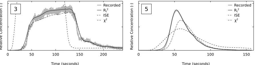
Figure 4 illustrates the poor performance of the χ2 and ISE constraints in contrast to
233
R2
t, before solution convergence. χ2 roughly matches the shape but not scale and ISE only
234
roughly matches shape. The performance of these two constraints does not improve with
235
more iterations while the performance of the R2t constraint does, which is typical of the other
236
remaining constraints, R2, RMSD, and APE.
237
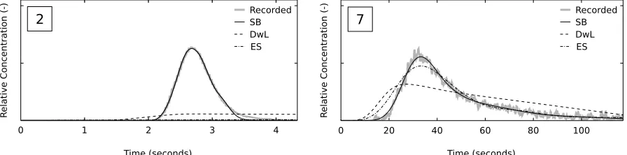
Figure 3 also suggests that the DwL and ES sample point distributions perform poorly,
238
and therefore these two distributions were eliminated from further consideration. Figure 5
239
confirms the elimination of DwL and ES by comparison to the SB distribution. Only the SB
240
distribution fits the data for both Experiments 2 and 7. The other two distributions result
241
in approximate fits for Experiment 7 only. For Experiment 2, DwL is mostly flat and ES is
242
almost entirely coincident with the x-axis. This highlights the impact of poor sample point
243
distribution choice.
244
The difference in DwL performance between Experiment 2 and 7 highlights the potential
245
unreliability of sample point distributions when assumptions made in developing the
dis-246
tribution are not met. For DwL at low numbers of sample points, the 6 fixed points leave
247
too few (only 4) points to characterize the curve. Additionally, due to the lower limits of
248
detection and the effects of noise, the first arrival time identified from the concentration
249
data will be coincident or later than the actual RTD peak. This results in too few points to
250
correctly capture the rising limb of the RTD, leading to the observed poor performance.
251
After eliminating BLC, χ2, ISE, FFCBS, DwL, and ES as configuration options, the
252
mean R2 values indicate improving goodness-of-fit for maximum number of iterations up to
150 iterations and near constant performance thereafter. As such, 50 and 100 iterations were
254
also eliminated, at which point it was observed that mean R2 also tended to increase with
255
number of sample points. Although this is not evident in Figure 3, R2 increases until 80
256
sample points, then remains close to constant. Due to their low mean R2, 10 and 20 sample
257
points have been eliminated as well.
258
All 4,000 remaining R2 values exceed 0.95, and 68.6% exceed 0.99. Differences in mean R2
259
value are less than 0.002, and as such there is very little sensitivity of goodness-of-fit to the
260
remaining options. This demonstrates the robustness of maximum entropy deconvolution
261
for most combinations of 40-200 sample points, the LFZ, DuL, SB, and DC distributions,
262
the R2, RMSD, R2
t, and APE constraints, and 150-350 iterations.
263
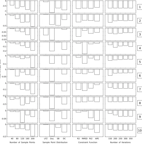
Entropy values
264
Entropy values have been examined to further evaluate RTD sensitivity to configuration
265
option. Mean entropy values for each experiment with respect to each option are shown in
266
Figure 6. These are plotted individually as entropy is a dimensional measure. The figure
267
provides insight into the sensitivity of the deconvolved RTD to the different options the
268
configuration settings can take.
269
40 sample points results in the entropy closest to zero for 9 of 10 experiments, which
270
clearly recommends 40 sample points and therefore other numbers of sample points can be
271
eliminated from consideration. The general trend of entropy values further from zero for
272
increased number of sample points is consistently observed independently of dataset. A
273
greater number of sample points provides increased potential for entropy as each sample
274
point represents a possible change in the slope of the RTD.
275
The LFZ and SB distributions appear to perform almost identically across all
experi-276
ments, with entropy values significantly closer to zero than the DuL and DC distributions
277
for almost all experiments. The entropy values further from zero indicate that, although the
278
DuL and DC distributions will generate RTDs with high goodness-of-fit, the shape of the
279
RTDs is less smooth. They are indicated to be less robust and can therefore be eliminated
from consideration.
281
Number and distribution of sample points have the highest impact on entropy and
there-282
fore on the quality of the deconvolved RTD. This is consistent with the problem formulation,
283
i.e. changes in sample point position affect the numerical problem being solved. Although
284
there are multiple RTD solutions for each experiment, improved sample point positioning
285
(and lower numbers of sample points) limits variation and results in smoother RTDs. That
286
R2 values remain high in these cases demonstrates the robustness of maximum entropy
de-287
convolution as applied to solute transport.
288
There is no clear trend in constraint function, with high variation between experiments.
289
The smaller changes in entropy with respect to constraint are reasonable considering that
290
constraints are interchangeable measures of error. As all of the constraint functions, R2,
291
RMSD, R2
t, and APE, are indicated to be perform similarly they are retained for further
292
examination.
293
Entropy values are closer to zero as the maximum number of iterations increases for
294
Experiments 2, 5, and 6. The opposite trend is shown by Experiments 7, 9, and 10.
Exper-295
iments 1, 3, 4, and 8 show no clear trend. Typically, however, more iterations allows for a
296
better solution to be reached, with either entropy closer to zero or increased goodness-of-fit.
297
Therefore, 350 iterations can be recommended and lower maximum numbers of iterations
298
eliminated from consideration. Higher numbers of sample points require comparatively more
299
iterations to reach entropy values closer to zero. Maximum number of iterations has the
low-300
est impact on entropy performance, which indicates that most RTDs reach convergence.
301
Mass-balance performance
302
Performance has been further examined by comparing the mass-balance of the remaining
303
deconvolved RTDs. The LFZ and SB distributions have been compared, using 40 sample
304
points, the remaining four constraint functions, and 350 iterations. The SB distribution
305
performs better, with all values close to 1, and therefore LFZ has been eliminated from
306
consideration. The mass-balance performance shows no systematic variation with respect to
constraint function.
308
Recommended configuration options
309
There is some evidence in the entropy data presented in Figure 6 that the paired
ex-310
periments from each of the five datasets responded similarly to the four different constraint
311
functions; this suggests that the optimal constraint function may be linked to dataset
char-312
acteristics. However, general investigation and consideration of all results suggests that the
313
R2
t constraint may perform slightly better. An additional argument in favour of R2t would
314
be that it is already a well used and understood measure in the field of solute transport.
315
Therefore the new SB sample point distribution, 40 sample points, 350 iterations, and the
316
R2t constraint function have been identified as a robust set of configuration options.
317
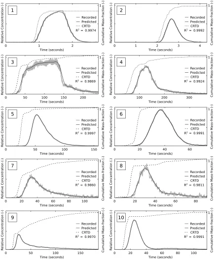
VALIDATION 318
Predicted downstream profiles and CRTDs generated with the robust configuration
op-319
tions (40 sample points, the new SB distribution, the R2t constraint, and 350 iterations) are
320
shown in Figure 7. The lower than expected final value of the CRTD for Experiment 1 is
321
the result of the poor mass-recovery of the laboratory concentration data (Table 1). The
322
predicted profiles give confidence that the identified configuration options are fit for use in
323
deconvolution, with mean R2 = 0.994.
324
CONCLUSIONS 325
Maximum entropy deconvolution has previously been successfully applied to laboratory
326
solute transport data to identify the residence time distribution from laboratory data. Here,
327
we have used laboratory data to evaluate the impact of four different configuration settings
328
on the deconvolved RTD. These settings are the number and distribution of sample points,
329
the constraint function, and the maximum number of iterations.
330
The smoothness of the deconvolved RTD, evaluated by entropy, is particularly sensitive
331
to number and distribution of sample points. A greater number of sample points provides
332
increased potential for noise as each point is a possible change in slope of the RTD. Smaller
numbers of sample points therefore tend to result in a smoother RTD, as well as reduced
334
computational expense. However, too few or poorly positioned sample points will result
335
in a poor quality RTD. A new slope-based sample point distribution, where sample points
336
are positioned based on an Fast-Fourier Transform deconvolution approximation, has been
337
proposed and shown to perform best out of the 6 tested sample point distributions.
338
The constraint function affects the overall goodness-of-fit between the recorded
down-339
stream concentration profile and a predicted profile generated using the deconvolved RTD,
340
here evaluated by R2. While maximum entropy deconvolution has typically utilized χ2 as
341
the constraint function, alternative correlation measures place different emphasis on
match-342
ing profile shape, scale, or noise. The present analysis suggests that χ2 does not provide a
343
robust constraint for solute transport data, but that the R2, RMSD, R2
t, and APE constraint
344
functions do. There is some evidence that the optimal constraint function may be linked to
345
specific data set characteristics, but as it is well understood in the field of solute transport,
346
R2t has been recommended as the most generically applicable constraint function.
347
Finally, we have shown that a maximum number iterations greater than 200 has a
min-348
imal impact on either the R2 value or RTD smoothness. However, performance in some
349
cases continues to increase maximum number of iterations and so 350 iterations has been
350
recommended here. RTD smoothness results imply that the vast majority of deconvolutions
351
reach convergence before the maximum number of iterations is reached.
352
Across ten representative laboratory solute transport data, the recommended
configu-353
ration options – 40 sample points, the new slope-based sample point distribution, the R2t
354
constraint function, and a maximum of 350 iterations – result in a mean R2 value for the
355
predicted downstream profiles of 0.994. This confirms that maximum entropy deconvolution
356
with the options recommended here provides a robust and effective means of identifying the
357
RTD from laboratory solute transport data.
358
Anderson, M. and Woessner, W. (1992). Applied groundwater modeling: simulation of flow 360
and advective transport.Academic Press, Inc., London.
361
Blackman, R. B. and Tukey, J. W. (1958). The measurement of power spectra, from the 362
point of view of communications engineering. Dover books on engineering and engineering
363
physics. Dover Publications.
364
Cirpka, O. A., Fienen, M. N., Hofer, M., Hoehn, E., Tessarini, A., Kipfer, R., and
Ki-365
tanidis, P. K. (2007). “Analyzing bank filtration by deconvoluting time series of electric
366
conductivity.” Ground Water, 45(3), 318–328.
367
Davis, P. M., Atkinson, T. C., and Wigley, T. M. L. (2000). “Longitudinal dispersion in
368
natural channels: 2. The roles of shear flow dispersion and dead zones in the River Severn,
369
UK.” Hydrology and Earth System Sciences Discussions, 4(3), 355–371.
370
Fan, Y., Sarkar, S., and Lasdon, L. (1988). “Experiments with successive quadratic
program-371
ming algorithms.”Journal of Optimization Theory and Applications, 56(3), 359–383.
372
George, S., Burnham, K., and Mahtani, J. (1998). “Modelling and simulation of hydraulic
373
components for vehicle applications - a precursor to control system design.” Simulation 374
’98. International Conference on (Conf. Publ. No. 457), 126 –132 (sep-2 oct).
375
Ghosh, A. K. (2007).Intro. to Linear & Digital Control Systems. Prentice-Hall Of India Pvt.
376
Ltd.
377
Gooseff, M. N., Benson, D. A., Briggs, M. A., Weaver, M., Wollheim, W., Peterson, B., and
378
Hopkinson, C. S. (2011). “Residence time distributions in surface transient storage zones
379
in streams: Estimation via signal deconvolution.” Water Resources Research, 47.
380
Guymer, I. (1998). “Longitudinal dispersion in sinuous channel with changes in shape.”
381
Journal of Hydraulic Engineering, 124(1), 33–40.
382
Guymer, I., Dennis, P., O’Brien, R., and Saiyudthong, C. (2005). “Diameter and surcharge
383
effects on solute transport across surcharged manholes.”Journal of Hydraulic Engineering-384
Asce, 131(4), 312–321.
385
Guymer, I., Shepherd, W. J., Dearing, M., Dutton, R., and Saul, A. J. (2002). “Solute
tion in storage tanks.” Proceedings of 9th International Conference on Urban Drainage, 387
Portland, Oregon, USA.
388
Guymer, I. and Stovin, V. R. (2011). “One-dimensional mixing model for surcharged
man-389
holes.”Journal of Hydraulic Engineering, 137(10), 1160–1172.
390
Harris, F. J. (1978). “On the use of windows for harmonic analysis with the discrete fourier
391
transform.” Proceedings of the IEEE, 66(1), 51–83.
392
Hart, J., Guymer, I., Jones, A., and Stovin, V. R. (2013). “Longitudinal dispersion
co-393
efficients within turbulent and transitional pipe flow.” Experimental and Computational 394
Solutions of Hydraulic Problems, P. Rowinski, ed., Springer.
395
Hattersley, J. G., Evans, N. D., Hutchison, C., Cockwell, P., Mead, G., Bradwell, A. R.,
396
and Chappell, M. J. (2008). “Nonparametric prediction of free-lightchain generation in
397
multiple myelomapatients.” 17th International Federation of Automatic Control World 398
Congress (IFAC), Seoul, Korea, 8091–8096.
399
Kashefipour, S. and Falconer, R. (2000). “An improved model for predicting sediment fluxes
400
in estuarine waters.”Proceedings of the Fourth International Hydroinformatics Conference, 401
Iowa, USA.
402
Levenspiel, O. (1972). Chemical Reaction Engineering. John Wiley & Son, Inc.
403
Madden, F. N., Godfrey, K. R., Chappell, M. J., Hovorka, R., and Bates, R. A. (1996). “A
404
comparison of six deconvolution techniques.” Journal of Pharmacokinetics and Biophar-405
maceutics, 24(3), 283–299.
406
Nash, J. E. and Sutcliffe, J. V. (1970). “River flow forecasting through conceptual models
407
part I - A discussion of principles.” Journal of Hydrology, 10(3), 282–290.
408
Pandolfi, L. (2010). “On-line input identification and application to active noise
cancella-409
tion.”Annual Reviews in Control, 34(2), 245–261.
410
Rieckermann, J., Neumann, M., Ort, C., Huisman, J. L., and Gujer, W. (2005). “Dispersion
411
coefficients of sewers from tracer experiments.” Water Science and Technology, 52(5),
412
123–133.
Rutherford, J. C. (1994). River mixing. John Wiley & Son Ltd, Chichester, England.
414
Sherman, L. K. (1932). “Streamflow from rainfall by the unit-graph method.” Engineering 415
News Record, 108, 501–505.
416
Skaggs, T. H., Kabala, Z. J., and Jury, W. A. (1998). “Deconvolution of a nonparametric
417
transfer function for solute transport in soils.”Journal of Hydrology, 207(3-4), 170–178.
418
Skilling, J. and Bryan, R. K. (1984). “Maximum-entropy image-reconstruction - general
419
algorithm.”Monthly Notices of the Royal Astronomical Society, 211(1), 111–124.
420
Sonnenwald, F., Stovin, V., and Guymer, I. (2011). “The influence of outlet angle on solute
421
transport in surcharged manholes.” 12th International Conference on Urban Drainage.,
422
Porte Alegre, Brazil.
423
Sonnenwald, F., Stovin, V. R., and Guymer, I. (2013). “Correlation measures for solute
424
transport model identification & evaluation.” Experimental and Computational Solutions 425
of Hydraulic Problems, P. Rowinski, ed., Springer.
426
Stovin, V., Guymer, I., and Lau, S. D. (2010a). “Dimensionless method to characterize the
427
mixing effects of surcharged manholes.” Journal of Hydraulic Engineering, 136(5), 318–
428
327.
429
Stovin, V. R., Guymer, I., Chappell, M. J., and Hattersley, J. G. (2010b). “The use of
decon-430
volution techniques to identify the fundamental mixing characteristics of urban drainage
431
structures.”Water Science and Technology, 61(8), 2075–2081.
432
Stovin, V. R., Guymer, I., and Lau, D. (2007). “Cumulative concentrations modelling
longi-433
tudinal dispersion - an upstream temporal concentration profile-independent approach.”
434
Proceedings of The 5th International Symposium on Environmental Hydraulics, Tempe,
435
Arizona.
436
Taylor, G. (1954). “The dispersion of matter in turbulent flow through a pipe.” Proceedings 437
of the Royal Society of London. Series A: Mathematical and Physical Sciences, 223(1155),
438
446–468.
439
The MathWorks Inc. (2011). MATLAB R2011a. Natick, MA.
The Morgridge Institute for Research (2012). “Sequential quadratic programming,
441
<http://www.neos-guide.org/content/sequential-quadratic-programming> (July. 18,
442
2012).
443
Ye, J. C., Tang, Y., Peng, H., and Zheng, Q. L. (2004). “FFCBS: A simple similarity
mea-444
surement for time series.”Proceedings of the 2004 International Conference on Intelligent 445
Mechatronics and Automation, 392–396.
446
Young, P., Jakeman, A., and McMurtrie, R. (1980). “An instrumental variable method for
447
model order identification.”Automatica, 16(3), 281–294.
448
Zhong, W. J., Wang, D. H., Xu, X. W., Wang, B. Y., Luo, Q., Senthil Kumaran, S., and
449
Wang, Z. J. (2011). “A gas chromatography/mass spectrometry method for the
simultane-450
ous analysis of 50 phenols in wastewater using deconvolution technology.”Chinese Science 451
Bulletin, 56(3), 275–284.
List of Tables 453
1 Summary of laboratory solute transport concentration data used. . . 20
TABLE 1. Summary of laboratory solute transport concentration data used.
Experiment Description Flow (l/s)* Duration (s) Mass recovery
1 24 mm Pipe1 1.084 150.0 84.42%
2 24 mm Pipe1 0.221 150.0 98.45%
3 Storage Tank2 6.9 240.2 100.00%
4 Storage Tank2 6 371.6 100.00%
5 Natural Channel3 13.7 157.3 101.96%
6 Trapezoidal Channel3 46.1 73.7 105.60%
7 400 mm BT Manhole4 1 117.3 100.00%
8 400 mm AT Manhole4 1 91.0 100.00%
9 800 mm BT Manhole5 1 186.0 100.00%
10 800 mm AT Manhole5 1 116.7 100.00%
1Hart et al. (2013),2Guymer et al. (2002),3Guymer (1998)
List of Figures 455
1 Example sample point distributions using 40 sample points. . . 22
456
2 Upstream and downstream concentration profiles of experiments. Time origin
457
set to 0 and Experiment 1 and 2 zoomed in for display. . . 23
458
3 Mean (µ) and standard deviation (σ) of R2 values by configuration option. . 24
459
4 Predicted downstream profiles with deconvolved RTDs using 40 sample points,
460
the SB sample point distribution, 50 iterations, and the χ2, R2t, or ISE
con-461
straint for Experiments 3 and 5. . . 25
462
5 Predicted downstream profiles with deconvolved RTDs using 10 sample points,
463
the DwL, ES, or SB sample point distribution, 350 iterations, and the R2 t
464
constraint for Experiments 2 and 7. . . 26
465
6 Mean entropy values by experiment and configuration option. Min R2 =
466
0.950, mean R2 = 0.994. . . 27
467
7 Predicted downstream profiles and deconvolved CRTDs for each experiment. 28
R
el
a
tive
C
o
n
cen
tr
at
ion
(
-)
Time (seconds)
0 20 40 60 80 100 120 140 160 180
DC SB DuL DwL LFZ ES
RTD
DC SB DuL DwL LFZ ES
[image:23.612.79.534.283.431.2]160 180 Upstream Downstream Sample Point
R el a tive C on cen tr at ion ( -) Time (seconds)
0 1 2
R el a tive C on cen tr at ion ( -) Time (seconds)
0 50 100 150 200
R el a tive C on cen tr at ion ( -) Time (seconds)
0 20 40 60 80 100
R el a tive C on cen tr at ion ( -) Time (seconds)
0 50 100 150 Upstream Downstream R el a tive C on cen tr at ion ( -) Time (seconds)
0 50 100 150
Upstream Downstream Upstream Downstream Upstream Downstream R el a tive C on cen tr at ion ( -) Time (seconds)
1 2 3 4
0 R el a tive C on cen tr at ion ( -) Time (seconds)
0 100 200 300
R el a tive C on cen tr at ion ( -) Time (seconds)
0 20 40 60 80
R el a tive C on cen tr at ion ( -) Time (seconds)
0 20 40 60 80 100 Upstream Downstream Upstream Downstream R el a tive C on cen tr at ion ( -) Time (seconds)
0 20 40 60
[image:24.612.95.520.70.591.2]Upstream Downstream Upstream Downstream Upstream Downstream 1 Upstream Downstream 2 3 4 6 5 7 8 10 9
σ(R
2)
0 0.2 0.4
μ(R
2) 0.5
1
10 20 40 80 120 160 200 LFZ
DwL DuL ES SB DC BLC χ
2
FF
C
B
S 2R
RMSD
Rt
2
ISE APE 50 100 150 200 250 300 350
[image:25.612.75.547.277.434.2]Number of Sample Points Sample Point Distribution Constraint Function Number of Iterations
R
el
a
tive C
on
cen
tr
at
ion
(
-)
Time (seconds)
0 50 100 150 200
Rt2
ISE χ2
Recorded
R
el
a
tive C
on
cen
tr
at
ion
(
-)
Time (seconds)
0 50 100 150
Rt2
ISE χ2
Recorded
[image:26.612.84.531.284.398.2]3 5
FIG. 4. Predicted downstream profiles with deconvolved RTDs using 40 sample points,
the SB sample point distribution, 50 iterations, and the χ2, R2t, or ISE constraint for
R
el
a
tive C
on
cen
tr
at
ion
(
-)
Time (seconds)
SB DwL ES Recorded
R
el
a
tive C
on
cen
tr
at
ion
(
-)
Time (seconds)
0 20 40 60 80 100
SB DwL ES Recorded
0 1 2 3 4
[image:27.612.83.531.286.397.2]2 7
FIG. 5. Predicted downstream profiles with deconvolved RTDs using 10 sample points,
the DwL, ES, or SB sample point distribution, 350 iterations, and the R2t constraint
-1 -0.5 0
-0.5 0
-0.03 -0.02 -0.01
-0.2 -0.1 0
-0.1 0
Mea
n
E
n
tr
opy V
alu
e
-0.05 0
-0.2 -0.1 0
-0.5 0
40 80 120 160 200
-0.05
R2 RMSD Rt2 APE
0
Number of Sample Points Constraint Function
-0.5 0
150 200 250 300 350
Number of Iterations
LFZ DuL SB DC
Sample Point Distribution
1
2
3
4
6 5
7
8
[image:28.612.77.556.108.595.2]10 9
FIG. 6. Mean entropy values by experiment and configuration option. Min R2 = 0.950,
R el a tive C on cen tr at ion ( -) Time (seconds) R el a tive C on cen tr at ion ( -) Time (seconds)
0 50 100 150 200
Time (seconds) R el a tive C on cen tr at ion ( -) Time (seconds)
0 20 40 60 80 100
R el a tive C on cen tr at ion ( -) Time (seconds)
0 50 100 150
R el a tive C on cen tr at ion ( -)
0 50 100 150
1 1 1 1 1 C u mu lat ive Ma ss -fr ac ti on ( -) C u mu lat ive Ma ss -fr ac ti on ( -) C u mu lat ive Ma ss -fr ac ti on ( -) C u mu lat ive Ma ss -fr ac tion (-) C u mu lat ive Ma ss -fr ac ti on ( -) CRTD Recorded Predicted
R2 = 0.9974
CRTD Recorded Predicted
R2 = 0.9869
CRTD Recorded Predicted
R2 = 0.9997
CRTD Recorded Predicted
R2 = 0.9860
CRTD Recorded Predicted
R2 = 0.9970
0 1 2
1 3 5 7 R el a tive C on cen tr at ion ( -) Time (seconds) R el a tive C on cen tr at ion ( -) Time (seconds)
0 100 200 300
Time (seconds) R el a tive C on cen tr at ion ( -) Time (seconds)
0 20 40 60 80
R el a tive C on cen tr at ion ( -) Time (seconds)
0 20 40 60 80 100
R el a tive C on cen tr at ion ( -)
0 20 40 60
1 1 1 1 1 C u mu lat ive Ma ss -fr ac ti on ( -) C u mu lat ive Ma ss -fr ac ti on ( -) C u mu lat ive Ma ss -fr ac ti on ( -) C u mu lat ive Ma ss -fr ac tion (-) C u mu lat ive Ma ss -fr ac ti on ( -) CRTD Recorded Predicted
R2 = 0.9992
CRTD Recorded Predicted
R2 = 0.9924
CRTD Recorded Predicted
R2 = 0.9991
CRTD Recorded Predicted
R2 = 0.9811
CRTD Recorded Predicted
R2 = 0.9991
1 2 3 4
[image:29.612.89.525.72.601.2]0 2 4 6 8 10 9