Coupling and the policy improvement algorithm for controlled diffusion processess

(1)

University of Warwick institutional repository: http://go.warwick.ac.uk/wrap

A Thesis Submitted for the Degree of PhD at the University of Warwick

http://go.warwick.ac.uk/wrap/73446

This thesis is made available online and is protected by original copyright.

Please scroll down to view the document itself.

(2)

Coupling and the policy improvement

algorithm for controlled diffusion processes

by

Dejan ˇ

Siraj

Thesis

Submitted to the University of Warwick

for the degree of

Doctor of Philosophy

Department of Statistics

(3)

Acknowledgments

First I would like to thank my parents, not only for their unconditional support

during my studies, but also for everything they did for me before that, in particular

for encouraging my curiosity. A big thank you also goes to my brother Mitja –

among other things, it has been really convenient to have free accommodation in

central London at any time.

I am most grateful to my supervisors, Professor Saul Jacka and Dr Aleksandar

Mijatovi´c, for their guidance, support and advice, always coupled with a good deal

of patience. Under their mentorship, it has been really rewarding to learn how

Mathematics is being made and presented.

Furthermore, I would like to thank my friends and colleagues, both in

Eng-land and Slovenia, for mutual support, fruitful discussions, all the fun moments,

those little pieces of advice about LA_{TEX or Matlab that save you a huge amount of}

time, and much more.

Special thanks go to all my teachers – I would not have been able to start the

PhD without the previously acquired skills and knowledge. In particular, I would

like to thank Professor Matjaˇz Omladiˇc for delivering my first course on probability,

being my undergraduate theses supervisor, and supporting my decision to pursue

my doctorate abroad.

Finally, I would like to thank the Slovene Human Resources Development

and Scholarship Fund for their scholarship. I am also grateful to the Department

of Statistics, University of Warwick, not only for the partial bursary award, but

also for providing stimulating and friendly research environment, for giving me an

(6)

Declarations

This thesis is submitted to the University of Warwick in support of my application

for the degree of Doctor of Philosophy. It has been composed by myself and has not

been submitted in any previous application for any degree.

Chapters 2, 3 and 4 are joint work with my supervisors Prof. S. D. Jacka and

Dr A. Mijatovi´c. The content of Chapters 3 and 4 is in preparation for publication,

whereas the content of Chapter 2 has been published as follows:

• S. D. Jacka, A. Mijatovi´c and D. ˇSiraj, Mirror and Synchronous Couplings of Geometric Brownian Motions. Stochastic Processes and their Applications,

(7)

Abstract

The thesis deals with the mirror and synchronous couplings of geometric

Brownian motions, the policy improvement (or iteration) algorithm in completely

continuous settings, and an application where the latter is applied to the former.

First we investigate whether the mirror and synchronous couplings of

Brow-nian motions minimise and maximise, respectively, the coupling time of the

cor-responding geometric Brownian motions. We prove (via Bellman’s principle) that

this is indeed the case in the infinite horizon and ergodic average problems, but not

necessarily in the finite horizon and exponential efficiency problems, for which we

characterise when the two couplings are suboptimal.

Then we describe the policy improvement algorithm for controlled diffusion

processes in the framework of the discounted infinite horizon problem, both in one

and several dimensions. Under some assumptions on the data of the problem, we

prove that the algorithm yields a sequence of Markov policies such that its

accu-mulation point is an optimal policy, and that the corresponding payoff functions

converge monotonically to the value function. We use no discretisation procedures

at any stage. We show that a large class of data satisfies the assumptions, and an

example implemented in Matlab demonstrates that the convergence is numerically

fast.

Next we study the policy improvement algorithm for continuous finite horizon

problem. We obtain analogous results as for the infinite horizon problem. Finally we

apply the algorithm to a certain sequence of data to approximate the value function

(8)

Chapter 1

Introduction

1.1 Structure of the thesis

1.1.1 Structure of this chapter

In Section 1.2 we present the basic coupling terminology and prove the coupling inequality. Then we investigate the mirror coupling of Brownian motions. This

par-ticular example was chosen not only because it illustrates well the newly introduced

concepts, but also because it prepares the ground for the next chapter, in which we deal with the same type of problems but for more complex processes. The section

closes with a short literature review on coupling.

Section 1.3 introduces the policy improvement algorithm in a simple set-ting. We treat the discrete discounted infinite-horizon minimisation problem with

countable state space and finite action space. We prove that the algorithm indeed improves the policy at each step. Although the treatment of the policy improvement

algorithm in Chapters 3 and 4 will be quite different and more involved, this simple

exposition manages to convey the main idea behind the algorithm concisely, which is why it is included. The section again ends with a brief literature review.

1.1.2 Structure of the rest of the thesis

Chapter 2 investigates whether the mirror and synchronous couplings of geometric

Brownian motions are optimal in four different (although related) problems. Chap-ter 3 presents the policy improvement algorithm for the discounted infinite-horizon

problem in a continuous setting. In the final chapter we make a connection between

(9)

The three chapters have a similar structure. First comes the introduction,

where the problems that will be treated in the chapter are motivated. Then most of the subsequent sections deal with one of them. Statement of the problem and the

result(s) are always in an independent subsection for greater transparency. They

are followed by the proof(s) in either one or two subsections, depending on whether extensive auxiliary results are required. Each chapter ends with the conclusion,

which includes a very brief summary, certain observations and comparisons,

rea-sons why the assumptions had or had not been made, comments about possible generalisations, and other remarks.

The numbering of theorems, lemmas, assumptions, etc., is unified. It includes

the chapter number, section number, and the consecutive number of the theorem, lemma, assumption, etc., in that section.

1.2 Coupling

1.2.1 Terminology and the coupling inequality

This subsection is very standard, see e.g. [22] or [30].

Let ( ˆΩ,F,ˆ _Pˆ) and ( ˆΩ0,Fˆ0,Pˆ0) be probability spaces, (E,E) a measurable

space, ˆX : ˆΩ → E an ( ˆF,E)-measurable mapping, and ˆX0 : ˆΩ0 → E an ( ˆF0,E )-measurable mapping. A coupling of random elements ˆX and ˆX0 is an (F,E ⊗ E )-measurable mapping (X, X0) : Ω→E×E such that

X= ˆL X and X0 L= ˆX0,

where (Ω,F,P) is a probability space and= denotes the equality in law (i.e. distri-L

bution).

The coupling where we make the random elements independent always exists

due to the product space construction. However, usually we want some dependence

because such couplings can be more informative.

(10)

measurable space (E,E) is defined as1

||P−Q||:= sup

A∈E

|P(A)−Q(A)|.

Let for any random elementX the symbolPX denote the law ofX.

The following lemma, called the coupling inequality, provides an upper bound for the total variation distance between the laws of the coupled random elements.

Note that the left-hand side does not depend on the coupling (i.e. the joint law)

whereas the right-hand side does.

Lemma 1.2.1. Let (E,E) be a Polish2 space, Xˆ and Xˆ0 random elements on it, and(X, X0) their coupling, which is defined on the probability space(Ω,F,P). Then

||P_X_ˆ −P_Xˆ0|| ≤P(X 6=X0).

Proof. For anyA∈ E we obtain

P_Xˆ(A)−P_Xˆ0(A) =P(X ∈A)−P(X0 ∈A)

=P(X ∈A, X 6=X0) +P(X∈A, X =X0)

−_P(X0∈A, X 6=X0)−_P(X0∈A, X =X0) =P(X ∈A, X 6=X0)−P(X0 ∈A, X 6=X0)

≤P(X ∈A, X 6=X0)

≤_P(X 6=X0).

By symmetry we get|P_X(A)−PX0(A)| ≤_P(X 6=X0), and by taking the supremum

overA∈ E the desired inequality follows.

IfX andX0are stochastic processes with the index setI ⊆_R, their coupling 1

Some authors define the total variation distance between the probability measuresPandQas 2 sup_A∈E|P(A)−Q(A)|since this expression is equal to

sup

Z

E

XdP−

Z

E

XdQ

; X:E→[−1,1] is (E,B([−1,1]))-measurable

.

2 _{In fact the space (}_E,_E_{) does not have to be Polish (i.e. separable and completely metrizable),}

only the diagonal has to be measurable, i.e.

(11)

timeτ is defined as

τ = inf{t∈I; Xs=Xs0 for all s≥t}, (inf∅:=∞).

The random time τ is neither necessarily a stopping time (with respect to either

of the natural filtrations) nor an almost surely finite random variable. We say that

coupling is successful ifτ is almost surely finite.

Since the inclusion{X_t6=X_t0} ⊆ {τ > t} holds for everyt∈I, the coupling inequality implies

||PXt−PX_t0|| ≤P(τ > t), t∈I.

Coupling of stochastic processesX and X0 is called maximal if equality is achieved

in the previous inequality for every t ∈ I. See [30, Ch. 3] for a comprehensive treatment of maximal couplings.

1.2.2 The mirror coupling of Brownian motions

The content of this subsection is well-known, see e.g. [13] or [22].

Let (Ω,F,(Ft)t≥0,P) be a filtered probability space that supports an (Ft)t≥0 -Brownian motion B = (Bt)t≥0. (Brownian motion in this thesis will mean one-dimensional Brownian motion started at 0, unless stated otherwise.) Let V be the set of all (F_t)t≥0-Brownian motions. Letx1, x2 ∈R, and for any V ∈ V define

τ(V) := inf{t≥0; x1+Bt=x2+Vt}, (inf∅:=∞).

For anyT >0, we would like to solve the following problem:

find B−∈ V such that inf

V∈VP(τ(V)> T) =P(τ(B

−₎_{> T}₎_. _(P)

Remark 1.2.2. The analogous maximisation problem, i.e.

find B+∈ V such that sup

V∈VP

(τ(V)> T) =P(τ(B+)> T),

has an obvious solution B+ ₌_B _since _τ₍_B_{) =} _∞ _if _x

1 6= x2. We call (B, B) the synchronous coupling of Brownian motions.

(12)

and not necessarily their coupling time. However, if we define the processV by

Vt:=

 



Vt if t∈[0, τ(V)], Bt if t∈(τ(V),∞),

then the following become apparent: V ∈ V since bothB andV are strong Markov processes with respect to the same filtration,τ(V) =τ(V), andτ(V) is the coupling

time ofB and V. Therefore by Lemma 1.2.1, Problem (P) is equivalent to finding

a maximal coupling of two (Ft)t≥0-Brownian motions started at x1 and x2. The following theorem provides a solution.

Theorem 1.2.3. For anyx1, x2∈RandT >0, a solution to Problem (P)is given

by

B−=−B.

Remark 1.2.4. It follows from the proof that the coupling (x1 +B, x2 +−B) is maximal and successful. It is usually called the mirror (or reflection) coupling of (one-dimensional) Brownian motions started atx1 and x2, however we will refer to

(B,−B) as the mirror coupling of Brownian motions.

Proof. It is enough to prove that the coupling inequality becomes equality for the

mirror coupling, i.e.

||P_x₁₊_B_t−Px2−Bt||=P(τ(−B)> t), t≥0.

We can assumex1< x2 without loss of generality. Note

τ(−B) = inf

t >0; Bt=

x2−x1 2

,

and therefore

P(τ(−B)> t) =P

sup

s≤t Bs<

x2−x1 2

=P

|B_t| ≤ x2−x1

2

, t≥0,

by the Reflection Principle.

On the other hand we have the following:

˜

A:=

y∈_R; e−(x12−ty)2 ≥e−

(x₂−y)2 2t

=

y ∈_R; y≤ x1+x2

2

(13)

Hence we obtain

||Px1+Bt−Px2−Bt||= sup

A∈B(R)

|P(x1+Bt∈A)−P(x2−Bt∈A)|

= sup

A∈B(R)

(P(x1+Bt∈A)−P(x2−Bt∈A))

= √1

2πtA∈B(supR)

Z

A

e−(x1

−y)2

2t −e−

(x2−y)2 2t

dy

= √1

2πt

Z

˜

A

e−(x1

−y)2

2t −e−

(x2−y)2 2t

dy

= √1

2πt

Z x1+₂x2

−∞

e−(x1

−y)2

2t dy− √1

2πt

Z x1+₂x2

−∞

e−(x2

−y)2 2t dy

= √1

2πt

Z x2−x1

2

−∞ e−y

2

2t dy−√1

2πt

Z x1−x2

2

−∞ e−y

2

2t dy

=P

Bt≤

x2−x1 2

−P

Bt≤

x1−x2 2

=P

|Bt| ≤

x2−x1 2

, t≥0.

1.2.3 Literature review

Coupling is a very useful technique, and a popular topic in probability. See the

classical books [22] and [30] for the general theory and numerous applications.

The mirror and synchronous couplings of Brownian motions and related pro-cesses have attracted much attention in the literature. Paper [23] introduces the

mirror coupling of Brownian motions and diffusion processes. In [13] it is established

that the mirror coupling of Brownian motions is not the only maximal coupling, al-though it is the unique maximal coupling in the family of Markovian (or immersion)

couplings. More about the Markovian maximal couplings for diffusion processes can

be found in [2] and [19].

In [3] it is proved that the tracking error of two driftless diffusions is

min-imised by the synchronous coupling of the driving Brownian motions. In [15]

gen-eralised mirror coupling and gengen-eralised synchronous coupling of Brownian motions are introduced; the former minimises the coupling time and maximises the tracking

error of two regime-switching martingales, whereas the latter does the opposite.

(14)

efficiency of a Markovian coupling, also used in this thesis, is studied in the context

of the spectral gap of the generator of a Markov process.

1.3 Policy improvement algorithm

1.3.1 Discrete discounted infinite-horizon problem

The algorithm has become an established method. See [14] and [27] for reference. We are given the following data:

• the state spaceS, which is a countable (i.e. finite or denumerable) set;

• the action spaceA, which is a finite set;

• the discount factorα∈(0,1);

• the cost functionR:S×A→_R, which satisfies

sup

i∈S

max

a∈A|R(i, a)| ≤M

for someM ∈R(if the state space is finite, this condition holds automatically);

• the transition probabilities{Pi,j(a); i, j ∈S, a∈A}, which satisfy

∀i, j ∈S ∀a∈A:Pi,j(a)∈[0,1] and ∀i∈S ∀a∈A:

X

j∈S

Pi,j(a) = 1.

Now we define the following objects (for any sets C and D,CD _{is the set of}

all mappings fromDtoC):

• the set of Markov policies:

AM :=

π={π_k}_k∈N0; ∀k∈N0:πk∈A

S _;

• the set of stationary policies: A_S := AS; note that even though A_S is not a subset ofAM, we will treat it as such due to the following natural embedding: π7→(π, π,· · ·);

(15)

(we know that it exists) since we will actually only need the law of the

pro-cess{Xπ

k}k∈N0, which is unique givenX

π

0; note that if π∈ AS, the controlled

process is a time-homogeneous Markov chain with the transition matrix equal

to{P_i,j(π(i)); i, j ∈S};

• (for everyπ ∈ A_M) the payoff function Vπ :S →Rgiven by

Vπ(i) :=E

∞

X

k=0

αkR(X_kπ, πk(Xkπ))

X₀π =i

!

, i∈S;

note that it is well-defined since

∞

X

k=0

αk|R(X_kπ, πk(Xkπ))| ≤

∞

X

k=0

αkM = M 1−α;

• the value functionV :S→_R, defined by

V(·) := inf

π∈AM

Vπ(·);

note thatV is a bounded function due to the estimate above;

• the optimality equation, which is the following function equation (forv):

v(i) = min

a∈A



R(i, a) +α X

j∈S

Pi,j(a)v(j)



, i∈S;

• the shift operatorθ: for any sequencex ={x_k}_k∈N0 let the sequence x◦θ be defined as

(x◦θ)k:=xk+1, k∈N0.

The problem is to find the value function and an optimal policy, if it exists.

Policyπ∈ A_M is optimal ifVπ(·) =V(·).

The following theorem characterises the value function and optimal policy. We will not prove it (it can be found in [27, Ch. 2]), but we will also not use it in

the proof of Theorem 1.3.3, which is the main result of this section.

Theorem 1.3.1. The value function V is the unique bounded solution of the opti-mality equation. Moreover, if we define the stationary policy π as

π(i) := argmin

a∈A



R(i, a) +α X

j∈S

Pi,j(a)V(j)



(16)

then it is an optimal policy.

We will follow the convention that if the minimum can be achieved by several

arguments, then argmin is any of them.

Mimicking the above formula, for any stationary policyπ define

π0(i) := argmin

a∈A



R(i, a) +α X

j∈S

Pi,j(a)Vπ(j)



, i∈S. (1.1)

Isπ0 better thanπ, i.e. isVπ0 smaller thanV_π? Before we reveal the answer, we will

prove the following lemma.

Lemma 1.3.2. For any Markov policyπ the following holds:

Vπ(i) =R(i, π0(i)) +α

X

j∈S

Pi,j(π0(i))Vπ◦θ(j), i∈S.

In particular, for any stationary policyπ we have

Vπ(i) =R(i, π(i)) +α

X

j∈S

Pi,j(π(i))Vπ(j), i∈S.

Proof. We obtain

Vπ(i) =E

∞

X

k=0

αkR(X_kπ, πk(Xkπ))

X₀π =i

!

=R(i, π0(i)) +αE

∞

X

k=0

αkR X_kπ₊₁, πk+1(Xkπ+1)

X₀π =i

!

=R(i, π0(i)) +α

X

j∈S

E

∞

X

k=0

X₀π =i, X₁π =j

!

·_P(X₁π =j|X₀π =i)

=R(i, π0(i)) +α

X

j∈S

E

∞

X

k=0

X₁π =j

!

Pi,j(π0(i))

=R(i, π0(i)) +αX j∈S

E

∞

X

k=0

αkR

X_kπ◦θ,(π◦θ)k(Xkπ◦θ)

X₀π◦θ =j

!

Pi,j(π0(i))

=R(i, π0(i)) +αX j∈S

(17)

The following theorem establishes thatπ0 is indeed an improvement of π.

Theorem 1.3.3. For every stationary policy π the following holds:

Vπ0(·)≤V_π(·).

Proof. For everyn∈_N₀ define the Markov policyπ(n) by

π_k(n)(i) =

 



π0(i) if k≤n, π(i) if k > n,

i∈S, k∈N0.

We will now show by induction thatV_π(n)(·)≤Vπ(·) holds for every n∈N0. First

we notice thatπ(0)◦θ=π. Using Lemma 1.3.2 and the definition ofπ0 in (1.1), we obtain

V_π(0)(i) =R(i, π0(i)) +α

X

j∈S

Pi,j(π0(i))Vπ(j)

= min

a∈A



R(i, a) +α X

j∈S

Pi,j(a)Vπ(j)





≤R(i, π(i)) +αX j∈S

Pi,j(π(i))Vπ(j)

=Vπ(i), i∈S.

Now suppose that V_π(m)(·) ≤ Vπ(·) holds for some m ∈ N0. Using the observation

π(m)◦θ=π(m−1)(ifm≥1), Lemma 1.3.2, the induction hypothesis and the previous inequality, we obtain

V_π(m+1)(i) =R(i, π0(i)) +α

X

j∈S

Pi,j(π0(i))Vπ(m)(j)

≤R(i, π0(i)) +αX j∈S

Pi,j(π0(i))Vπ(j)

=V_π(0)(i)

≤Vπ(i), i∈S,

which concludes the induction.

(18)

and boundedness ofR:

Vπ0(i)−V

π(n)(i) =_E ∞

X

k=0

αkRX_kπ0, π0(X_kπ0)

X₀π0 =i

!

−E

∞

X

k=0

αkRX_kπ(n), π_k(n)(X_kπ(n))

X₀π(n) =i

!

=E

∞

X

k=n+1

αkR

X_kπ0, π0(X_kπ0)

X₀π0 =i

!

−_E

∞

X

k=n+1

αkR X_kπn, π_kn(X_kπn)

X₀πn =i

!

≤2 ∞

X

k=n+1

αkM

= 2M α

n+1

1−α , i∈S, n∈N0.

To finish the proof, we note

Vπ0(i)−V_π(i) =V_π0(i)−V

π(n)(i) +V_π(n)(i)−Vπ(i)≤

2M αn+1

1−α , i∈S, n∈N0,

and sendnto∞.

The policy improvement algorithm is now defined as follows: take a

station-ary policyπ0 and then

πn+1(·) := (πn)0(·), n∈N0.

If it happens for somen∈_N₀ that V_πn+1(·) =V_πn(·), thenV_πn clearly satisfies the

optimality equation and is therefore the value function (andπnan optimal policy) by

Theorem 1.3.1. In the case of the finite state spaceS this means that the algorithm always achieves an optimal policy (and usually this happens very quickly). In the

general case the following theorem states that the sequence{Vπn}_n_∈

N0 converges to the value function.

Theorem 1.3.4. For any initial stationary policy π0, the sequence {Vπn}_n_∈

N0

con-verges uniformly to V.

(19)

We will prove that the statement

Vπn(i)≤V(i) + ˜M αn, i∈S

holds for every n ∈ _N₀, which implies the theorem. Assume that the statement holds for somem∈_N0. Then we obtain

Vπm+1(i)

Lemma 1.3.2

= R(i, πm+1(i)) +αX j∈S

Pi,j(πm+1(i))Vπm+1(j)

Thm. 1.3.3

≤ R(i, πm+1(i)) +αX j∈S

Pi,j(πm+1(i))Vπm(j)

PIA = min

a∈A



R(i, a) +α X

j∈S

Pi,j(a)Vπm(j) 



I.H.

≤ min

a∈A



R(i, a) +α X

j∈S

Pi,j(a)(V(j) + ˜M αm)





Thm. 1.3.1

= V(i) + ˜M αm+1, i∈S,

which conludes the induction and hence the proof.

1.3.2 Literature review

Since Howard’s book [12] containing the policy improvement (or policy iteration)

algorithm was published in 1960, a lot of work has been done on this subject. A survey of approximate policy iteration methods for finite state, discrete time,

stochastic dynamic programming problems is given in [4]. The algorithm has proved to be useful in deterministic control theory, too (see e.g. [8] and [31]). Nevertheless,

it has probably been applied most often to Markov decision processes in various

settings (see [7], [10], [11], [21], [25], [20], [24], [28], [29] and [32]).

Most of the settings of the above papers are discrete, but some are continuous

(or general) to a certain extent. For example, article [7] deals with continuous time

Markov decision processes on a fairly general state space, but the policy improvement algorithm is only proved to work in the special case of finite action space. Paper [32]

removes this restriction, but even there the controlled processes are not continuous.

(20)

Chapter 2

Mirror and synchronous

couplings of geometric

Brownian motions

2.1 Introduction

Recall that in Subsection 1.2.2 we solved the following finite horizon problem for

any T >0:

minimise/maximise P(τ(V)> T) over all Brownian motions V,

where τ(V) is the first meeting time of the processes x+B and y+V, x, y ∈ _R, and B and V are Brownian motions with respect to the same filtration (and B is

considered to be fixed). We proved that a solution is given by the mirror coupling (i.e. an optimal Brownian motion is V =−B) in the case of minimisation, and by the synchronous coupling (i.e. an optimal Brownian motion is V =B) in the case

of maximisation. Since the solution is the same for everyT >0, the two couplings must also solve the problems obtained by replacing the expression P(τ(V) > T)

above by

Z ∞

0

e−qtP τ(V)> tdt, (q >0),

lim sup

T→∞ 1

T

Z T

0

P(τ(V)> t) dt,

and

lim inf

t→∞ 1

(21)

which are called the infinite horizon problem, ergodic average problem and

expo-nential efficiency problem, respectively.

It is natural to investigate the analogous problems for other processes,

espe-cially geometric Brownian motions. In this caseτ(V) is the first meeting time of the

processes X and Y(V), whereX is a geometric Brownian motion started atx and driven byB, and Y(V) is a geometric Brownian motion started at y and driven by

V. SinceXtandY(V)tare at any timetgiven by explicit deterministic functions of Bt andVtrespectively, we might expect that the mirror and synchronous couplings

of B and V will again be optimal in the finite horizon problem. However, as we

shall see, this turns out to be false in general. Consequently, the other problems are

not trivial, and we will look into them, too.

An application in mathematical finance of the finite horizon problem

consid-ered in the present chapter can be described as follows. Assume that the

perfor-mance of a portfolio manager is assessed at some fixed future time (e.g. one year from now) with respect to a benchmark security (e.g. some equity index), which

evolves as a geometric Brownian motion X. Put differently, the remuneration of

the manager depends on whether their portfolio, which evolves as Y(V), exceeds the benchmark X in normalised terms. Assume also that the manager’s mandate

stipulates that, over the same time horizon, their portfolio may not exceed a pre-specified amount of realised variance. Both of these assumptions are realistic and are

used extensively in practice, since the investor wants to beat the index but cannot

tolerate arbitrary amounts of volatility in the meantime (e.g. investors like pension funds routinely stipulate such realised variance conditions). Imagine now a situation

where the manager has a given amount of time, sayT, before the evaluation of their

performance, but is behind the benchmark by a certain amount. The question of how to trade in such a way as to minimise the probability of not catching up with

the benchmark before T, and to achieve this without taking unnecessary bets that

would increase the realised volatility of the portfolio, is precisely the question of the stochastic minimisation of the first meeting time betweenX and Y(V) (recall that

the expected quadratic variation ofY(V), i.e. the realised variance of the manager’s

portfolio, does not depend on the choice of Brownian motionV).

In the next section we describe the setting and basic notation, which remain

throughout the chapter. We also state a lemma from stochastic analysis, which

enables us to apply Bellman’s principle, on which some of the proofs are based. Then each of the four sections deals with one of the above problems. In Sections 2.3

and 2.5 we prove that the mirror and synchronous couplings always solve the infinite

(22)

that two couplings are not always optimal for the finite horizon and exponential

efficiency problem, respectively, and provide a characterisation of when exactly this happens.

2.2 Setting and notation

Let (Ω,F,(Ft)t≥0,P) be a filtered probability space satisfying the usual conditions

that is rich enough to support an (F_t)-Brownian motionB = (Bt)t≥0, and set

V :={V = (Vt)t≥0; V is an (Ft)-Brownian motion}.

The following well-known lemma will come in useful. For its proof, see e.g. [15,

Lemma 2.1].

Lemma 2.2.1. For any Brownian motion V ∈ V, there exists an (F_t)-Brownian motion W ∈ V and a process C = (Ct)t≥0 such that B and W are independent, C

is progressively measurable with −1≤Ct≤1 for all t≥0 P-a.s., and the following

representation holds:

Vt=

Z t

0

CsdBs+

Z t

0

p

1−C2

sdWs, t≥0.

Remark 2.2.2. The proof of this lemma requires the existence of a Brownian motion

B⊥ ∈ V that is independent of B. If our probability space did not support such a Brownian motion, we could enlarge it, which would only increase the set V. This means that if B and −B are optimal in the new problem, they also have to be optimal in the original problem. Therefore we can assume thatB⊥ exists.

For any V ∈ V, let X = (Xt)t≥0 and Y(V) = (Yt(V))t≥0 be geometric Brownian motions given by the following stochastic differential equations:

Xt=x+

Z t

0

Xs(σ1dBs+a1ds), Yt(V) =y+

Z t

0

Ys(V) (σ2dVs+a2ds), (2.1)

where

x, y >0, a1, a2∈R, and σ1, σ2 ∈R such that σ1σ2 >0. (2.2)

Define the following constants:

(23)

Note that (2.2) implies|σ₊|>|σ−|. The symbol±denotes either + or −. If±and

∓appear in the same expression, then they simultaneously denote either + and−, or−and +.

Defineτ(V) as the first meeting time of the two processes in (2.1), i.e.

τ(V) := inf{t≥0; Xt=Yt(V)} (inf∅:=∞).

The random variableτ(V) is zero when the two processes start at the same point and

positive P-a.s. otherwise. Since the filtration (Ft)t≥0 satisfies the usual conditions,

τ(V) is an (Ft)-stopping time. SinceX andY(V) are geometric Brownian motions,

this stopping time has the following useful representation:

τ(V) = inf

t≥0; log

x y

=σ2Vt−σ1Bt+µt

. (2.4)

2.3 Infinite horizon problems

2.3.1 The problems and main theorem

For anyq >0, we consider the following two problems: find Vinf ∈ V and Vsup ∈ V

(if they exist) such that

inf

V∈V

Z ∞

0

e−qtP τ(V)> tdt=

Z ∞

0

e−qtP τ Vinf> tdt (qInf)

and

sup

V∈V

Z ∞

0

e−qtP τ(V)> tdt=

Z ∞

0

e−qtP τ(Vsup)> tdt. (qSup)

An application of Fubini’s theorem (or integration by parts for Riemann-Stieltjes integral) yields

Z ∞

0

e−rtP(τ > t) dt= 1

−_E(e−rτ)

r

for any nonnegative random variable τ and r > 0. Therefore Problems (qInf) and (qSup) are equivalent to finding V(+) _{∈ V} _and _V(−) _{∈ V} _{respectively, such} that

sup

V∈V

±E

e−qτ(V)

=±E

e−qτ(V(±))

. (q±)

Note also that ifeqis an exponential random variable withE(eq) = 1_q, independent of

(24)

The following theorem holds.

Theorem 2.3.1. A solution to Problem (q±) is (for anyq >0) given by

V(±)=∓B.

Remark 2.3.2. Observe that by Theorem 2.3.1, the mirror coupling (V(+) = −B) solves Problem (qInf) and the synchronous coupling (V(−)= +B) is the solution to

Problem (qSup). Note that the solution depends neither on the parameters in (2.2) nor on the discount rateq.

2.3.2 Proof

Note that, due to the symmetry in Problem (q±), we may assume without loss of generality that the starting points x, y in (2.1)–(2.2) satisfy (x, y) ∈ D, where the setD is given by

D:={(a, b)∈R2; a≥b >0}. (2.5)

Fixq >0 and define the following function, closely related to the right-hand side in

Problem (q±):

Ψ(±)(x, y) :=Ex,y

e−qτ(∓B), (x, y)∈D. (2.6)

The proof of Theorem 2.3.1 is in two steps: we first establish sufficient conditions

for a function Ψ : D → R+ implying that ±Ψ is equal to the right-hand side in Problem (q±) (Lemmas 2.3.3 and 2.3.4), and then prove that Ψ(±) in (2.6) satisfies these conditions (Lemma 2.3.5). Throughout the thesis we denoteR+:= [0,∞).

For any measurable function Ψ : D → R+ and Brownian motion V ∈ V, consider the processU(V,Ψ) = (Ut(V,Ψ))t∈[0,∞) defined by

Ut(V,Ψ) := e−q(t∧τ(V))Ψ(Xt∧τ(V), Yt∧τ(V)(V)) (2.7)

(here and in the rest of the thesis we denotes∧t:= min({s, t})). Then the following lemma (a suitable version of Bellman’s principle) holds.

Lemma 2.3.3. Let Ψ : D → _R₊ be a bounded continuous function satisfying

Ψ(x, x) = 1 for all x > 0. If, for every (x, y) ∈D, the process ±U(V,Ψ) is a Px,y -supermartingale for allV ∈ V andU(∓B,Ψ)is a Px,y-martingale, thenV(±)=∓B solves Problem (q±).

(25)

supermartingale property and the Dominated Convergence Theorem imply

±Ex,y

e−qτ(V)

=Ex,y ±Uτ(V)(V,Ψ)I{τ(V)<∞}

≤Ex,y(±U0(V,Ψ)) =±Ψ(x, y),

for all (x, y) ∈ D and V ∈ V (I{·} denotes the indicator of the event {·}). Since

U(∓B,Ψ) is a martingale, for V(±)=∓B this inequality becomes an equality and the lemma follows.

Our next task is to establish a verification lemma for Problem (q±). LetD◦

be the interior (inR2) of the setD defined in (2.5). For any functionf ∈ C2,2(D◦)

we define the functionL(±)f by the formula

L(±)f(x, y) :=

a1xfx+a2yfy +

1 2σ

2

1x2fxx+

1 2σ

2

2y2fyy∓σ1σ2xyfxy−qf

(x, y),

(2.8)

where (x, y) ∈ D◦ and fx, fy, fxx, fyy and fxy denote the partial derivatives of f.

For any function Ψ :D→R+such that Ψ∈ C2,2(D◦), and Brownian motionV ∈ V, the local martingaleM(V,Ψ) = (Mt(V,Ψ))t∈[0,∞), given by

Mt(V,Ψ) :=

Z t∧τ(V)

0

e−qsσ1XsΨx(Xs, Ys(V)) dBs

+

Z t∧τ(V)

0

e−qsσ2Ys(V)Ψy(Xs, Ys(V)) dVs,

(2.9)

is well-defined.

Lemma 2.3.4. Assume the following hold:

(I) Ψ :D→_R+ is a bounded continuous function withΨ(x, x) = 1for all x >0;

(II) Ψ∈ C2,2₍_D◦₎ _{and, in the interior} _D◦_, _Ψ

xy ≤0 and L(±)Ψ = 0; (III) M(V,Ψ) is aPx,y-martingale for all (x, y)∈D andV ∈ V.

Then for any (x, y) ∈ D, V ∈ V, the process ±U(V,Ψ), defined in (2.7), is a

Px,y-supermartingale and U(∓B,Ψ) is a Px,y-martingale.

Proof. The definition ofXandY(V) in (2.1) and Lemma 2.2.1 imply d[X, Y(V)]t= Ctσ1Xtσ2Yt(V) dt, where C = (Ct)t∈[0,∞) is (Ft)-adapted and P(Ct ∈ [−1,1]) = 1

(26)

ofU(V,Ψ) yield

±Ut(V,Ψ)

=±Ψ(x, y)±Mt(V,Ψ) +

Z t∧τ(V)

0

e−qsσ1σ2(1±Cs)XsYs(V)Ψxy(Xs, Ys(V)) ds

for all (x, y)∈Dand V ∈ V. Since X,Y(V) and 1±C are non-negative processes and, by assumption (2.2), we have σ1σ2 > 0, the integrand in the representation of±U(V,Ψ) is non-positive, making ±U(V,Ψ) a Px,y-supermartingale. For∓B we

haveCs=∓1 for everys≥0, which implies thatU(∓B,Ψ) is aPx,y-martingale.

Note the following equivalence:

Px,y(τ(∓B) =∞) = 1 for all (x, y)∈D◦ ⇐⇒ ∓= +, σ2 =σ1, a2 ≤a1. (2.10) It is clear that under condition (2.10) Theorem 2.3.1 holds. Lemmas 2.3.3 and 2.3.4

imply that in order to establish Theorem 2.3.1 in general, it is sufficient to prove

that, when (2.10) fails, the function Ψ(±):D→R+in (2.6) satisfies the assumptions of Lemma 2.3.4. More precisely, the following lemma holds.

Lemma 2.3.5. If for some (x, y) ∈ D◦ we have Px,y(τ(∓B) = ∞) < 1, Assump-tions (I)–(III) of Lemma 2.3.4 hold for the functionΨ(±):D→_R₊ in (2.6). Proof. Under the assumption of the lemma, the following representation holds:

Ψ(±)(x, y) =y

x

k±

, (x, y)∈D, (2.11)

where

k±:=

 



−µ/σ2

±+

q

(µ/σ2_±)2_{+ 2}_q/σ2

± if σ±6= 0,

q/µ if σ±= 0,

andσ±andµare defined in (2.3). Since, by assumption, the condition on the

right-hand side in (2.10) is not satisfied, the equality σ± = 0 impliesµ > 0, making k± a well-defined real number. Formula (2.11) follows from the fact thatτ(∓B) equals the first passage time of the Brownian motion with drift, (∓σ±Bt+µt)t∈[0,∞), over the level log

x y

. The Laplace transform of this random time is given in [5, p. 295] and amounts to the right-hand side of (2.11).

Assumption (I) in Lemma 2.3.4 follows from (2.11). Furthermore it is clear

(27)

that for (x, y)∈D◦ the following holds:

Ψ(±)_x (x, y) =−k± x Ψ

(±)₍_{x, y}₎_, _Ψ(±)

y (x, y) = k±

y Ψ

(±)₍_{x, y}₎_, _(2.12)

and

Ψ(±)_xy (x, y) =−k

2 ±

xy Ψ

(±)₍_{x, y}₎_≤₀_, _L(±)_Ψ(±)₍_{x, y}_{) = 0}_.

Hence assumption (II) of Lemma 2.3.4 is also satisfied. The equalities in (2.12) and

the definition in (2.9) of the local martingaleM(V,Ψ(±)) imply that the integrands in the stochastic integrals are bounded processes and therefore square integrable.

Hence M(V,Ψ(±)) is a Px,y-martingale for all (x, y) ∈ D and V ∈ V and

assump-tion (III) of Lemma 2.3.4 also holds.

2.4 Finite horizon problems

For anyT >0, consider the following problem(s):

findV(±) ∈ V such that inf

V∈V±Px,y τ(V)> T

=±_P_x,y τ V(±)

> T

. (T±)

Unlike in the infinite horizon problem, the mirror and synchronous couplings

are not always optimal. The following theorem characterises precisely when this is the case. Recall that µand σ± are given in (2.3), and Din (2.5).

Theorem 2.4.1. The following holds for any T >0 and (x, y)∈D◦: (a) ifµ >0 and σ±6= 0, then V(±)=∓B does NOT solve Problem (T±);

(b) if µ≤0, then V(±)=∓B solves Problem (T±).

Remark 2.4.2. In the case µ > 0 and σ± = 0 we have ± = −, σ1 = σ2 and Φ(−)(x, y, t) =I{tµ<log(x/y)} for all (x, y)∈D◦,t∈[0, T] (recall (2.4)), which implies that the synchronous coupling is suboptimal if and only ifT ≥ 1

µlog

x y

.

Remark 2.4.3. Intuition behind this theorem follows from the representation in (2.4):

starting from 0, we want to hit a positive level in a given time with as high probability

as possible (for the minimisation problem); when the drift is against us (i.e. non-positive), we are desperate and therefore choose the maximal variance at every

moment, which corresponds to the mirror coupling; when the drift is helping us,

(28)

in the case 0 < x < y, the theorem still holds if µ gets the opposite sign in the

statement.

2.4.2 Proof

Define the setE :=D×[0, T] and recall that the value function for Problem (T±) is defined by

F(x, y, t) := inf

V∈V±Px,y(τ(V)> t), (x, y, t)∈E. (2.13) Define also

Φ(±)(x, y, t) :=Px,y(τ(∓B)> t), (x, y, t)∈E, (2.14)

andA(±)_f _{for any} _f _{∈ C}2,2,1₍_E◦_{) (}_E◦ _{is the interior of}_E _in

R3) by the formula

A(±)f

(x, y, t) :=

a1xfx+a2yfy+

1 2σ

2

1x2fxx+

1 2σ

2

2y2fyy∓σ1σ2xyfxy−ft

(x, y, t),

where (x, y, t)∈E◦ and fx, fy, ft, etc., denote the partial derivatives off. For any

sufficiently smooth function Φ : E → _R₊ and any Brownian motion V ∈ V, we define the local martingaleN(V,Φ) = (Nt(V,Φ))t∈[0,T]by

Nt(V,Φ) :=

Z t∧τ(V) 0

σ1XsΦx(Xs, Ys(V), T−s) dBs

+

Z t∧τ(V)

0

σ2Ys(V)Φy(Xs, Ys(V), T −s) dVs.

(2.15)

The following proposition provides the key ingredient in the proof of Theorem 2.4.1.

Proposition 2.4.4. Let a bounded function Φ :E →_R₊ satisfy:

(i) Φ(x, x, t) = 0for allx >0andt∈[0, T], andΦ(x, y,0) = 1for all(x, y)∈D◦; (ii) Φ∈ C2,2,1₍_E◦₎ _{and, in the interior} _E◦_{, the equality} _A(±)_{Φ = 0} _holds;

(iii) N(V,Φ) is a Px,y-martingale for all (x, y)∈D andV ∈ V. Then the following equivalence holds:

(29)

Proof. (⇒): The proof of this implication is analogous to that of Lemmas 2.3.3 (Bellman’s principle) and 2.3.4 (submartingale property) in Section 2.3. The process

±U(V,Φ) = (±U_t(V,Φ))_t∈[0,T], given by

Ut(V,Φ) := Φ(Xt∧τ(V), Yt∧τ(V)(V), T −t), (2.16)

is a Px,y-submartingale for any V ∈ V and (x, y) ∈ D (proof as in Lemma 2.3.4).

For anyt∈[0, T], the boundary conditions in assumption (i) imply

Ut(V,Φ) =Uτ(V)(V,Φ) = 0 Px,y-a.s. on {t≥τ(V)}.

Hence, for any (x, y) ∈ D and V ∈ V, the submartingale property yields the in-equality

±Px,y(τ(V)> T) =Ex,y ±UT(V,Φ)I{τ(V)>T}

=Ex,y(±UT(V,Φ)) ≥ ±_Ex,yU0(V,Φ) =±Φ(x, y, T).

As in Lemma 2.3.3, this establishes the implication (note that, unlike in Lemma 2.3.3, in this case we do not need, and in fact do not have, the

continu-ity of Φ onE).

(⇐): Assume that there exists (x0, y0, T0)∈ E◦ such that Φxy(x0, y0, T0)<0, and that ±Φ is the value function of Problem (T±). Bellman’s principle implies that the process±U(V,Φ), defined in (2.16), is a Px,y-submartingale for anyV ∈ V and

(x, y) ∈D. Using our assumption, we will construct a Brownian motion ˜V(±) ∈ V

such that±U( ˜V(±),Φ) fails to be a Px,y-submartingale (for any pair (x, y) ∈ D◦),

which will imply the proposition.

The continuity of Φxy implies that there existsr >0, such that Φxy is strictly

negative on the setK2 :=H2×[T0−2r, T0+ 2r]⊂E◦, where

H2 := [x0−2r, x0+ 2r]×[y0−2r, y0+ 2r].

Let

H1 := [x0−r, x0+r]×[y0−r, y0+r] and define the stopping timesτ₁(±) and τ₂(±) by:

(30)

τ₂(±):= inf{t∈[τ1, T]; (Xt, Yt(±B))∈/H2}, (inf∅:=T). Note that τ₁(±) ≤ τ₂(±) ≤ T Px,y-a.s. and Px,y(τ

(±) 1 < τ

(±)

2 ) > 0 (there is a slight abuse of notation in the definition ofτ₂(±) as it is assumed that the processY(±B), defined in (2.1), is driven by the Brownian motion±B as indicated, but started at the random timeτ₁(±) and point Y_τ(±)

1

(∓B); ditto for X).

Define the process ˜V(±)= ( ˜V_t(±))t∈[0,∞) by the following formula:

˜

V_t(±):=

Z t

0

∓I_{_s<τ(±)

1 }

±I_{_τ(±) 1 ≤s<τ

(±)

2 }

∓I_{_s_≥_τ(±)

2 }

dBs.

Note that ˜V(±) is an (Ft)-Brownian motion by L´evy’s characterisation theorem.

Itˆo’s formula on the stochastic interval [τ₁(±), τ₂(±)] and assumptions (i)–(iii) in the proposition imply the following representation:

Ex,y

±U τ₂(±)( ˜V

(±)_,_Φ) F_τ(±)

1

=±U

τ₁(±)( ˜V

(±)_,_Φ)

+Ex,y

Z τ₂(±)

τ₁(±)

2σ1σ2XsYs( ˜V(±))Φxy(Xs, Ys( ˜V(±)), T −s) ds

F τ₁(±)

!

.

The event

A:={τ₁(±) ∈(T0−r, T0+r), τ( ˜V(±))> T0+ 2r}

has a strictly positive probability and the integrand under the conditional expecta-tion is strictly negative on this event. We therefore find

Ex,y

±U τ₂(±)( ˜V

(±)

,Φ)

F_τ(±)

1

<±U τ₁(±)( ˜V

(±)

,Φ) on A

Px,y-a.s. This inequality contradicts thePx,y-a.s. inequality

Ex,y

±U τ₂(±)( ˜V

(±)_,_Φ) F_τ(±)

1

≥ ±U τ₁(±)( ˜V

(±)_,_Φ)_,

which follows from the optional sampling theorem applied to the bounded Px,y

-submartingaleU( ˜V(±),Φ). This concludes the proof.

We will now apply Proposition 2.4.4 to study the question of whether±Φ(±), defined in (2.14), is the value function for Problem (T±).

(31)

hold for the functionΦ(±) defined in (2.14). Furthermore, we have

Φ(±)_xy (x, y, t) =

2 logx_y−4µt xy(|σ±|

√ t)3 n





logx_y−µt |σ±|

√ t





+ 4µ 2 xyσ4 ± x y 2µ σ_±2

N   −log x y −µt |σ±|

√ t





for all(x, y)∈D◦ andt >0, whereN(·)is the standard normal distribution function andn(·) is its density.

Proof. The explicit formula for the distribution of the running maximum of a

Brow-nian motion with drift (see e.g. [5, p. 250]) yields the following representation of the

function in (2.14):

Φ(±)(x, y, t) =h(±)

log x y , t

for (x, y)∈D, (2.17)

where, for anyz≥0 ands >0, we define

h(±)(z, s) :=N

z−µs |σ±|

√ s −exp 2µz σ2 ± N

−z−µs |σ±|

√ s

. (2.18)

Simple (but tedious) calculations using this representation yield the properties

re-quired in assumptions (i)–(iii) of Proposition 2.4.4. Indeed, note that the partial

derivativesh(±)z ,h

(±)

zz and h

(±)

s take the following form (recalln0(x) =−xn(x)):

h(±)_z (z, s) = 2

|σ±|

√ sn

z−µs |σ±|

√ s

− 2µ σ2 ± exp 2µz σ2 ± N _−z₋ µs |σ±|

√ s

,

h(±)_zz (z, s) = 4sµ−2z (|σ±|

√ s)3 n

z−µs |σ±|

√ s

−4µ

2 σ4 ± exp 2µz σ2 ± N

−z−µs |σ±|

√ s

,

h(±)_s (z, s) =− z |σ±|s3/2

n

z−µs |σ±|

√ s

.

These formulae and the representation in (2.17) imply the formula for Φ(±)xy (x, y, t),

as well as assumptions (i) and (ii) of Proposition 2.4.4. The martingale property

of the process in (2.15) (i.e. assumption (iii) in Proposition 2.4.4) follows by Itˆo’s isometry from the fact that both functions

xΦ(±)_x (x, y, t) =h(±)_z

log x y , t

and yΦ(±)_y (x, y, t) =−h(±)_z

(32)

are bounded onE. This completes the proof of the lemma.

We are now ready to prove Theorem 2.4.1.

Proof of Theorem 2.4.1. (a) By Proposition 2.4.4 it suffices to show that for any

t >0 there exists (x, y) ∈ D◦ (see (2.5) for the definition of D) such that Φ(±)xy (x y, t)<0.

Define z := _| 1

σ±|

√

tlog

x y

> 0 and α := µ √

t

|σ±| > 0. Note that, since we

are allowed to choose the point (x, y) ∈ D◦ arbitrarily close to the diagonal half-line in the boundary of D, a Taylor expansion of order one of z 7→ n(z−α) and

z7→ N(−z−α) around z= 0, the representation of Φ(±)xy in Lemma 2.4.5 and the

inequality

αN(−α)< n(−α) (2.19) imply that Φ(±)xy (x, y, t) < 0 for some (x, y) ∈ D◦. To check (2.19), note that un(u) =−n0(u) and

αN(−α) =

Z ∞

α

αn(u) du <

Z ∞

α

un(u) du=n(−α).

(b) Assume first σ± 6= 0. Then the representation of Φ (±)

xy in Lemma 2.4.5 and

the assumption µ ≤ 0 imply Φ(±)xy ≥ 0 on E◦. Hence Proposition 2.4.4 yields the

theorem. If σ± = 0, we have ± = −, σ1 = σ2 and, by (2.4), it follows that Φ(−)(x, y, t) = 1 holds for all (x, y) ∈ D◦, t ∈ [0, T]. Hence −Φ(−) is the value function for Problem (T−), and the theorem is proved.

2.5 Ergodic average problems

We would like to solve the following problems: find Vinf ∈ V and Vsup ∈ V such that

inf

V∈Vlim sup_T_→∞ 1

T

Z T

0

P(τ(V)> t) dt= lim sup

T→∞ 1

T

Z T

0

P(τ(Vinf)> t) dt (EAInf)

and

sup

V∈V

lim sup

T→∞ 1

T

Z T

0

P(τ(V)> t) dt= lim sup

T→∞ 1

T

Z T

0

(33)

Note first that Fubini’s theorem and the Dominated Convergence Theorem imply

that the limit exists and has the following representation:

lim

T→∞ 1

T

Z T

0

P(τ(V)> t) dt= lim

T→∞E

τ(V)

T ∧1

=P(τ(V) =∞). (2.20)

A solution to these problems, independent of the values of the parameters of the

geo-metric Brownian motions in (2.1), is given in the following theorem. It is completely

analogous to the infinite time horizon case.

Theorem 2.5.1. The Brownian motions Vinf = −B and Vsup = B solve Prob-lems (EAInf) and (EASup) respectively.

2.5.2 Proof

The proof is rather short due to (2.20) and because we can apply the result obtained

for the finite horizon problem.

Proof of Theorem 2.5.1. As in Section 2.3 we may assume that, due to symmetry, the starting points ofX andY(V) satisfy (x, y)∈D. Ifx=y we haveτ(V) = 0 for all V ∈ V and Proposition 2.5.1 follows. So we can assume (x, y) ∈D◦ in the rest of the proof.

We first analyse the caseµ >0. By (2.20), Problems (EAInf) and (EASup)

are equivalent to findingV(±)∈ V such that

inf

V∈V±P(τ(V) =∞) =±P(τ(V (±)

) =∞). (S±)

The strong law of large numbers for Brownian motion (see e.g. [5, p. 53]), repre-sentation (2.4) and logx_y> 0 imply the equality Px,y(τ(V) = ∞) = 0 for every V ∈ V and Theorem 2.5.1 follows.

In the case µ ≤ 0, we return to the formulation of Problems (EAInf) and (EASup) above. Observe that Theorem 2.4.1(b) yields the optimal couplings

that minimise and maximise the probability P(τ(V) > t) for every t ≥ 0. Since

the couplings are independent of t, they also minimise and maximise the ergodic

(34)

2.6 Exponential efficiency problems

We would like to findV(±)∈ V such that:

inf

V∈V±lim inft→∞

log Px,y(τ(V)> t)

t =±lim inft→∞

log Px,y τ V(±)

> t

t . (EE±)

It turns out that the answer is a dichotomy, as in the finite horizon problem. Recall thatµ and σ± are given in (2.3), and Din (2.5).

Theorem 2.6.1. The following holds for any (x, y)∈D◦: (a) If µ >0, then V(±)=∓B does NOT solve Problem (EE±). (b) If µ≤0, then V(±)=∓B solves Problem (EE±).

2.6.2 Proof

Proof of Theorem 2.6.1. The second part of the theorem again follows from

Theo-rem 2.4.1. We will prove the first part in the following way: when we claim thatB

is not optimal we will show that−B is better, and vice-versa.

The following bounds hold for the standard normal distribution functionN(·) and its derivativen(·):

− z

1 +z2 n(z)≤N(z)≤ −

n(z)

z for any z <0. (2.21)

The first inequality follows from the identity

Z ∞

r

1 + 1

y2

e−y 2

2 dy= 1

r e

−r2

2 , r >0,

and the second is given in (2.19). Assume first thatσ±6= 0. Let

Z(t) :=

logx_y−µt |σ±|

√

t and Zb(t) :=

−logx_y−µt |σ±|

√ t ,

and note that for all larget >0 we haveZb(t)< Z(t)<0, and the equality

n(Z(t)) =

x y

2µ σ_±2

nZb(t)

(35)

holds. The representations in (2.17) and (2.18) imply

Φ(±)(x, y, t) =N(Z(t)) 1−

x y

2µ

σ2_± N(Zb(t))

N(Z(t))

!

. (2.23)

The inequalities in (2.21) yield

lim

t→∞ 1

tlog N(Z(t))

=− µ

2

2σ2±

. (2.24)

In order to deal with the second factor on the right-hand side of (2.23), we note the

following inequalities:

1−

x y

2µ

σ2_± N(Zb(t))

N(Z(t)) ≥1 + (1 +Z(t)

2₎ N(Zb(t))

n(Zb(t))Z(t)

≥1−1 +Z(t)

2

b

Z(t)Z(t);

they are a consequence of two applications of the second inequality in (2.21) and identity (2.22). Let the assumption

log

x y

> σ

2 +

2µ (2.25)

hold. Then we obtain

1− 1 +Z(t)

2

b

Z(t)Z(t) = 1

t

2µlog

x y

−σ±2

−_t22 log

x y

2

µ2₋ 1

t2log

x y

2 >0 for all large t >0,

and

lim

t→∞ 1

tlog 1−

1 +Z(t)2

b

Z(t)Z(t)

!

= 0. (2.26)

By (2.23) we have

N(Z(t)) 1−1 +Z(t)

2

b

Z(t)Z(t)

!

≤Φ(±)(x, y, t)≤N(Z(t)).

If the starting pointsx, ysatisfy (2.25), then (2.24), (2.26), the inequalities in the line above and the fact that the function log is increasing imply the following equality:

lim

t→∞ 1

tlog

Φ(±)(x, y, t)=− µ

2

2σ_±2 .

(36)

(x, y) ∈ D such that log

x y

∈ 0,σ

2

±

2µ

i

, define a Brownian motion with drift W±

and its first-passage time T±(z):

W_t±:=∓σ±Bt+µt, t≥0, and T±(z) := inf{t≥0; Wt±=z}, z∈R,

and note that Px,y(τ(∓B) > t) = P

T±

logx_y> t holds for any (x, y) ∈ D

(cf. (2.4)). Fix (x, y) ∈ D that violates assumption (2.25) and pick α0 < 0 and (x0, y0)∈D◦ such that the following holds:

log x0 y0 = log x y

−α0>

σ2₊

2µ.

Denote the constantq±:=P

W₁± < α0, T±

logx_y>1, which clearly satisfies

q±∈(0,1). The Markov property of W± at time 1 yields the following inequalities for allt >1:

Px,y(τ(∓B)> t) =P

T± log x y > t

≥q±P

T± log x y

−α0

> t−1

> q±P

T± log x y

−α0

> t

=q±Px0,y0(τ(∓B)> t).

Since (2.23) implies the boundPx,y(τ(∓B)> t) ≤N(Z(t)) for any (x, y)∈D◦, we

obtain

lim

t→∞ 1

t log (Px,y(τ(∓B)> t)) = limt→∞ 1

t log

Φ(±)(x, y, t)=− µ

2

2σ2±

, (2.27)

by the inequality above, our analysis under assumption (2.25) and the limit in (2.24). Definition (2.3) and assumption σ± 6= 0 imply |σ+| > |σ−| > 0 and hence

− µ2

2σ2

− <

− µ2

2σ2 +

. The mirror coupling is therefore not optimal for Problem (EE+)

since it has a strictly thicker exponential tail than the synchronous coupling. Like-wise, the synchronous coupling is not optimal for Problem (EE−), which requires the thickest possible exponential tail among all couplings, since it has a thinner tail

than the mirror coupling.

In the caseσ±= 0 we have σ1 =σ2 and, by (2.4), τ(B) = _µ1log

x y

. Hence

Px,y(τ(B)> t) = 0 for allt≥ _µ1log

x y

(37)

±= + (note that |σ₊|>0), we obtain

lim

t→∞ 1

tlog (Px,y(τ(B)> t)) =−∞<− µ2

2σ2₊ = limt→∞ 1

tlog (Px,y(τ(−B)> t)).

This inequality implies that the mirror (resp. synchronous) coupling is not optimal

for Problem (EE+) (resp. (EE−)).

Remark 2.6.2. It is the presence of the positive drift µ >0 that makes the mirror coupling suboptimal in Problem (T+) (see Theorem 2.4.1). The proof of

Theo-rem 2.6.1 suggests that if the drift is positive, it is in fact better (according to the

exponential efficiency criterion) to use the synchronous coupling. This naturally leads to the following conjecture.

Conjecture 2.6.3. If µ > 0, the synchronous (resp. mirror) coupling is optimal in Problem (EE+) (resp. (EE−)).

2.7 Conclusion

We have seen that, unlike in the case of Brownian motions, the mirror and syn-chronous couplings are not always a solution to the finite horizon problem for

geo-metric Brownian motions. Nevertheless, this does not prevent them from solving the

ergodic average and infinite horizon problems (for all discount rates). Interestingly, when it comes to the exponential efficiency, this problem is again not always solved

by the two couplings.

For the exponential efficiency problem, we at least have a more or less natural

conjecture (although we do not see any natural way of proving or disproving it). In

the case of the finite horizon problem, there seems to be no clear candidate. It may even happen that there is no optimal coupling since the supremum and infimum

need not be attained. In any case, we will at least “obtain” the value function at

the very end of the thesis via the policy improvement algorithm. In fact, this is where the motivation to start looking at the policy improvement algorithm in a

continuous setting came from.

Why did we only deal with geometric Brownian motions and not general diffusion processes (with the diffusion coefficients of the same sign)? The reason lies

in Lemma 2.3.5, where certain analytical properties of the candidate value functions

had to be verified. In the case of geometric Brownian motions, this was easy since we had obtained an explicit formula for the functions. If we had been dealing with

(38)

Chapter 3

The policy improvement

algorithm for the general

continuous discounted

infinite-horizon problem

3.1 Introduction

To the best of the author’s knowledge, nothing has been published about the policy improvement algorithm for controlled processes in continuous time with continuous

state space, continuous paths and general action space. In this and the next

chap-ter we deal with such processes, which become diffusion processes if controlled by Markov policies.

In the present chapter we investigate the discounted infinite-horizon

minimi-sation problem. In Section 3.2 we treat the one-dimensional case. The first idea, based on the discrete case formula in (1.1), was to define the policy at each step

(given an initial policy) by

πn+1(x) := argmin p∈A

(LpVπn(x)−α(x, p)Vπn(x) +f(x, p)), x∈(a, b), n∈N0,

whereA is the compact action space, Lp the infinitesimal generator corresponding

to action p, Vπn the payoff function generated by the Markov policy πn, α the

discounting function, f the cost function, and (a, b) the (possibly infinite) state space. (Note that we have an additional term; this is becauseαin the discrete case,

(39)

HJB equation (cf. [18, p. 12]), with a normalising multiplier such that the policies

no longer depend on the second derivative of the payoff function: for eachn∈N0,

πn+1(x) := argmin

p∈A

µ(x, p)

σ(x, p)2 V 0

πn(x)−

α(x, p)

σ(x, p)2 Vπn(x) +

f(x, p)

σ(x, p)2

, x∈(a, b),

whereµis the drift and σ the diffusion coefficient.

We solve the problem by finding a convergent subsequence of the sequence

{π_n}_n∈_Nwhose limit is an optimal policy, and by proving that the sequence of payoff functions{Vπn}n∈N converges to the value function of the problem; the convergence

is monotonic, so the policy on each step of the algorithm indeed improves the pre-vious one (as in the discrete case). No discretisation of time, action space or state

space is involved at any point.

In Section 3.3 we treat the multidimensional case. Although the results can

be applied to one dimension, they do not imply the results of the previous section.

The results of Section 3.2 are more general because they deal with domains other thanRand because we can use the normed HJB equation. Despite this the proofs

in the multidimensional case are not easier, in fact there is an additional property

that has to be proved. For the purpose of elliptic differential equations theory, we need to establish the continuity of the payoff functions in advance. We do that by

invoking the mirror coupling of multidimensional diffusions (Lemma 3.3.13).

In order to carry out our proof that the algorithm works, the data of the problem have to satisfy certain assumptions; in Section 3.4 we show that there

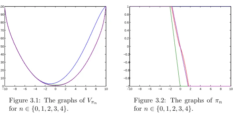
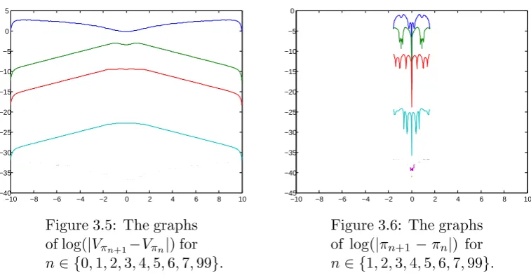
is a large family of suitable data. We also present a concrete example that we

implemented in Matlab, for which the convergence towards both the optimal policy and the value function is numerically very fast, which again sounds familiar from

the discrete case.

3.2 One-dimensional case

3.2.1 Setting and the algorithm

Let (Ω,F,(F_t)t≥0, P) be a filtered probability space (satisfying the usual conditions) that supports an (Ft)t≥0-Brownian motionB = (Bt)t≥0. Leta, b∈[−∞,∞], a < b,

and for anyR-valued process Y = (Yt)t≥0 define

(40)

Let (A, d) be a compact metric space, and for any x ∈ (a, b) define the set of admissible controls atx as

A(x) :={Π = (Πt)t≥0; Π is an A-valued process adapted to (Ft)t≥0, and there exists a pathwise unique process XΠ,x= X_tΠ,x_t_≥0 that satisfies (3.1)},

where

X_tΠ,x=x+

Z t

0

σ X_sΠ,x,Πs

dBs+

Z t

0

µ X_sΠ,x,Πs

ds, 0≤t < τ_ab XΠ,x, X_tΠ,x=X_τΠb,x

a(XΠ,x), τ

b a XΠ,x

≤t <∞,

(3.1)

and σ : (a, b)×A → _R and µ : (a, b)×A → _R are measurable functions. In fact it will not matter what the process XΠ,x looks like after it reaches a or b, if that occurs at all.

Letα : (a, b)×A→ _Rand f : (a, b)×A →_R be measurable functions and

g :{a, b} ∩_R→ _R an arbitrary function. For any x ∈ (a, b) and Π ∈ A(x) define the payoff as

VΠ(x) :=E

Z τ_ab(XΠ,x)

0

e−

Rt

0α(X Π,x s ,Πs)ds_f

X_tΠ,x,Πt

dt

+e−

Rτ ba(X

Π,x₎

0 α(X

Π,x t ,Πt)dt_g

X_τΠb,x a(XΠ,x)

I{τb

a(XΠ,x)<∞} !

.

The problem is to find thevalue function V, defined by

V(x) := inf

Π∈A(x)VΠ(x), x

∈(a, b),

and an optimal control (which will in general depend onx), if it exists.

In order to solve the problem, we make the following assumptions about the

functionsσ,µ,α and f.

Assumption 3.2.1. The functions σ, µ, α and f are bounded, and Lipschitz on

compacts in (a, b)×A, i.e. for every compact setK ⊆(a, b) there exists a constant

C >0 such that

|h(x, p)−h(y, r)| ≤C((x−y)2+d(p, r)2)12

(41)

Assumption 3.2.2. For everyh ∈ C2₍₍_{a, b}_{)) and} _x _∈₍_{a, b}_{), let} _I

h(x) denote a point

where the minimum of the function

p7→ µ(x, p) σ(x, p)2h

0₍_x₎₋ α(x, p)

σ(x, p)2 h(x) +

f(x, p)

σ(x, p)2, p∈A,

is attained. If the sequence {h0_n}n∈N is uniformly Lipschitz (i.e. there exists a

con-stant that is a Lipschitz concon-stant for all the functions in the sequence) on compacts

in (a, b), then the points{I_h_n(x); x∈(a, b), n∈_N}can be chosen in such a way that the sequence of functions{Ihn}n∈N (Ihn : (a, b)→A) is also uniformly Lipschitz on

compacts in (a, b).

Remark 3.2.3. It is important to note that there are non-trivial data that satisfy the above assumptions. Some are presented in Proposition 3.4.1.

We will need a special class of controls. A measurable functionπ: (a, b)→A

is a Markov policy if for every x ∈ (a, b) there exists a pathwise unique process

Xπ,x = (X_tπ,x)_t_≥0 that satisfies the following:

X_tπ,x =x+

Z t

0

σ(X_sπ,x, π(X_sπ,x)) dBs+

Z t

0

µ(X_sπ,x, π(X_sπ,x)) ds

if 0≤t < τ_ab(Xπ,x), X_tπ,x =X_τπ,xb

a(Xπ,x) if τ

b

a(Xπ,x)≤t <∞.

(3.2)

If π is a Markov policy, then π(Xπ,x) := (π(X_tπ,x))_t_≥0 ∈ A(x) for every x ∈ (a, b) (whereπ(a), ifa >−∞, andπ(b), ifb <∞, are arbitrary elements ofA). For easier notation we define

σπ(·) :=σ(·, π(·)), µπ(·) :=µ(·, π(·)), απ(·) :=α(·, π(·)), fπ(·) :=f(·, π(·)),

Vπ(·) :=Vπ(Xπ,·₎(·), and L_πh:= 1

2σ 2

πh

00

+µπh0 for h∈ C2((a, b)).

Ifπ is a constant Markov policy with the value p ∈A, we will write σp,µp,αp,fp

andLp instead ofσπ,µπ,απ,fπ and Lπ, respectively.

The first proposition establishes that there is a large class of Markov policies. It is the members of this class for which our algorithm will be defined. As explained

in Subsection 1.1.2, the proofs do not follow immediately, but are presented in the next two subsections.

Coupling and the policy improvement algorithm for controlled diffusion processess

University of Warwick institutional repository: http://go.warwick.ac.uk/wrap

A Thesis Submitted for the Degree of PhD at the University of Warwick

http://go.warwick.ac.uk/wrap/73446

This thesis is made available online and is protected by original copyright.

Please scroll down to view the document itself.

Coupling and the policy improvement

algorithm for controlled diffusion processes

Dejan ˇ

Siraj

Department of Statistics

Contents

Acknowledgments

Declarations

Abstract

Chapter 1

Introduction

1.1

Structure of the thesis

1.2

Coupling

1.3

Policy improvement algorithm

Chapter 2

Mirror and synchronous

couplings of geometric

Brownian motions

2.1

Introduction

2.2

Setting and notation

2.3

Infinite horizon problems

2.4

Finite horizon problems

2.5

Ergodic average problems

2.6

Exponential efficiency problems

2.7

Conclusion

Chapter 3

The policy improvement

algorithm for the general

continuous discounted

infinite-horizon problem

3.1

Introduction

3.2

One-dimensional case