warwick.ac.uk/lib-publications
Manuscript version: Author’s Accepted Manuscript
The version presented in WRAP is the author’s accepted manuscript and may differ from the
published version or Version of Record.
Persistent WRAP URL:
http://wrap.warwick.ac.uk/124205
How to cite:
Please refer to published version for the most recent bibliographic citation information.
If a published version is known of, the repository item page linked to above, will contain
details on accessing it.
Copyright and reuse:
The Warwick Research Archive Portal (WRAP) makes this work by researchers of the
University of Warwick available open access under the following conditions.
Copyright © and all moral rights to the version of the paper presented here belong to the
individual author(s) and/or other copyright owners. To the extent reasonable and
practicable the material made available in WRAP has been checked for eligibility before
being made available.
Copies of full items can be used for personal research or study, educational, or not-for-profit
purposes without prior permission or charge. Provided that the authors, title and full
bibliographic details are credited, a hyperlink and/or URL is given for the original metadata
page and the content is not changed in any way.
Publisher’s statement:
Please refer to the repository item page, publisher’s statement section, for further
information.
Design and Analysis of an Acknowledgment-Aware
Asynchronous MPR MAC Protocol for Distributed
WLANs
Arpan Mukhopadhyay, Neelesh B. Mehta, Senior Member, IEEE, Vikram Srinivasan, Member, IEEE
Abstract—Multi-packet reception (MPR) promises significant
throughput gains in wireless local area networks (WLANs) by allowing nodes to transmit even in the presence of ongoing transmissions in the medium. However, the medium access control (MAC) layer must now be redesigned to facilitate – rather than discourage – these overlapping transmissions. We investigate asynchronous MPR MAC protocols, which successfully accom-plish this by controlling the node behavior based on the number of ongoing transmissions in the channel. The protocols use the backoff timer mechanism of the distributed coordination function (DCF), which makes them distributed and practically appealing. We first highlight a unique problem of acknowledgment (ACK) delays, which arises in asynchronous MPR, and investigate a solution that modifies the medium access rules to reduce these delays and increase system throughput in the single receiver scenario. We develop a general renewal-theoretic fixed-point analysis of the solution and derive expressions for its saturation throughput, packet dropping probability, and average head-of-line packet delay. We also model and analyze the practical scenario in which nodes may incorrectly estimate the number of ongoing transmissions.
Index Terms—Cross-layer design, Medium access control,
Multi-packet reception, Wireless local area network, IEEE 802.11, Fixed-point analysis, Timer backoff
I. INTRODUCTION
Conventional wireless local area networks (WLANs), which use the IEEE 802.11 distributed coordination function (DCF) [1] and its enhancements as medium access control (MAC) protocols, are facing increasing demands for higher data rates and higher system throughput. Conventionally, a layered approach is adopted in designing the physical (PHY) and MAC layers. For example, the DCF MAC uses carrier sense multiple access (CSMA) with collision avoidance (CA) to discourage time-overlapping transmissions by multiple users in the uplink channel from the nodes to the AP. This is accomplished by making the nodes freeze their backoff timers anytime they sense an ongoing transmission in the channel.
With the advent of advanced signal processing techniques based on code division multiple access (CDMA), successive interference cancellation (SIC), or multiple antennas, today’s
A. Mukhopadhyay is with the Dept. of Electrical and Computer Eng. at the Univ. of Waterloo, Canada. N. B. Mehta is with the Dept. of Electrical Communication Eng. at the Indian Institute of Science (IISc), Bangalore, India. V. Srinivasan is with Bell Labs Research, Alcatel-Lucent, Bangalore, India. A. Mukhopadhyay was at IISc during the course of this work.
Emails: [email protected], [email protected]
A part of this work has been presented in the IEEE Global Communications Conf. (Globecom), USA, 2012.
wireless receivers are capable of decoding multiple simultane-ous transmissions. This has been referred to as the multi-packet reception (MPR) capability [2]–[9]. Instead of discouraging overlapping transmissions, the MAC layer must now facilitate their occurrence in order to benefit from MPR. At the same time, the MAC should retain the distributed manner in which nodes access the medium, as this is a key reason behind the success of the IEEE 802.11 DCF MAC.
A. Related Literature
We now summarize some key papers on MPR and ascertain their efficacy, distributed nature, and suitability for an IEEE 802.11-type DCF MAC. MPR was first considered in [8], [10] for slotted ALOHA, but CSMA was not modeled. An adaptive MAC protocol for MPR that maximizes the expected number of successfully transmitted packets per slot and also takes into account quality of service requirements was proposed in [5]. A simpler variant based on collision resolution was proposed in [11]. A similar objective was achieved in [4] for space division multiple access systems (SDMA) that use multiple antenna APs. However, these protocols require a central controller that selects an optimal set of users that access the channel in each slot.
A generic, distributed asynchronous MPR model, which exploited the fact that a multiple antenna node can estimate the number of ongoing transmissions, was recently analyzed by Babich and Comisso in [16] using Markov chains. In it, a node continues to decrement its backoff timer and eventually transmits even when it senses the channel to be busy – so long as the number of ongoing transmissions is less than or equal to a threshold; else, it freezes its timer. The protocol was ana-lyzed without any limitation on the number of receivers [17]. However, ACKs were not modeled; it was implicitly assumed that a node knows whether its transmission has succeeded or not immediately after transmitting its packet. Further, nodes were assumed to perfectly estimate the number of ongoing transmissions.
The use of MPR in an asynchronous set up can, in fact, delay the transmission of an ACK by the AP. This is because packet transmissions by different nodes can now start at differ-ent time slots and overlap without any idle period in between. Consequently, the AP will have to continue to receive packets even after a particular node completes its transmission. As a result, the transmission of an ACK by the AP, which is a half-duplex node, can get significantly delayed. Since the presence or absence of an ACK makes a node update its backoff parameters, ACK delays can degrade system throughput and increase packet transmission delays.
B. Contributions
The paper makes several contributions on the following aspects of asynchronous MPR MAC.
Protocol Design: The paper first points out that in an asynchronous MPR MAC protocol, ACKs may get delayed. This delay in the reception of ACKs, which is absent in con-ventional DCF and synchronous MPR protocols, can degrade the system performance. Thus, an asynchronous MPR MAC protocol needs to be designed keeping ACK delays in mind. To this end, we propose and compare two asynchronous MPR MAC protocols both of which incorporate ACKs in the single receiver scenario. The first protocol is our own interpretation of how ACKs can be incorporated in the model analyzed in [16], and serves as a benchmark. In the second protocol, the multiple access rules, which determine when a node should freeze or decrement its backoff timer, are modified to reduce the ACK delays and increase system throughput. In it, nodes freeze their backoff timers once the number of transmissions in the channel reaches the MPR capability of the AP or once any node completes the transmission of its packet. This ensures that a node, which has just finished transmitting its packet, waits for no more than one packet duration to receive an ACK. Modeling imperfect estimation: Another important contri-bution of the paper is a tractable modeling of the practical scenario where the nodes incorrectly estimate the number of ongoing transmissions in the channel. We show that the first and the second protocols are quite robust to imperfect estimation. Several MPR-specific implementation issues are also discussed.
Analysis: Finally, the paper develops a general, renewal-theoretic fixed-point analysis of the second asynchronous MPR
MAC protocol that explicitly takes ACKs into consideration. The analysis can handle the ideal case with perfect estimates and the practical case with imperfect estimates. Analytical expressions for the saturation throughput, packet dropping probability, and average head-of-line packet delay are derived. Saturation throughput is an important performance measure for a MAC protocol and has been extensively analyzed in the literature on conventional 802.11 DCF and MPR. It gives a limit on the system throughput in heavy traffic loads [6], [14], [15], [18], [19]. In some cases, it also provides a sufficient condition for stability of queues at the nodes [20]. The average head-of-line delay is also an important performance measure as it affects higher layers of the protocol stack and is the first step in a queueing delay analysis for a non-saturated traffic scenario [21], [22].
The renewal-theoretic approach developed in this paper is different from the Markovian analysis used in [16], [18]. For example, in our analysis, packet lengths need not follow the memoryless geometric probability distribution, which breaks down under heavy traffic load conditions when a packet suffers many retransmissions [16]. The effect of packet dropping after a finite number of retransmissions is also incorporated. Our analysis also generalizes the renewal-theoretic analysis that was developed in [19] for conventional DCF.
Performance benchmarking: We also extensively bench-mark the saturation throughput, head-of-line packet delay, and packet dropping probability of the two asynchronous MPR MAC protocols and conventional DCF. This is done for both ideal and imperfect estimation.
The paper is organized as follows. Section II sets up the system model and the asynchronous MPR MAC protocols, which are then analyzed in Section III. Imperfect estimation is modeled and analyzed in Section IV. Simulations results in Section V are followed by our conclusions in Section VI.
II. SYSTEMMODEL
A. System Model
Consider the uplink of a WLAN, in which the AP acts as the central node and n surrounding nodes need to transmit packets directly to the AP. The following MPR data reception model is assumed, along the lines of [6], [14], [16]. The AP can successfully decode all the overlapping transmissions as long as the number of overlapping transmissions is less than or equal toL. If more thanLoverlapping transmissions occur, then the AP fails to decode the transmissions and a collision is said to occur. Here,Lis called the MPR capability.1Further, it is assumed that a node can correctly estimate whether the num-ber of ongoing transmissions in the channel is0,1, . . . , L−1, or whether it is greater than or equal to L. Techniques to estimate the number of ongoing transmissions and the effect of imperfect estimates are discussed in Section IV.
Each node follows the timer-based binary exponential back-off scheme of conventional DCF, and a packet is dropped by a node after K+ 1 failed transmission attempts. Before each transmission attempt, a node selects its backoff period in
1This MPR reception capability based model can also be expressed in terms
DATA
DATA
DATA
A
B
C Backoff
freeze
R
ec
eive
C
u
mu
lat
ive
A
C
K
TDIFS
TSIFS
Wait to start ACK-timeout
Wait to start ACK-timeout
TSIFS
TSIFS
Backoff decrement
TDIFS
[image:4.612.83.265.55.214.2]TDIFS
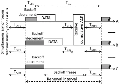
Fig. 1. Protocol 1 forL= 2: Timing diagram showing a renewal interval in which three overlapping asynchronous transmissions to the AP occur. NodeA
transmits first. NodesBandCcontinue to decrement their timers until node
Btransmits. Thereafter,Cfreezes its timer. WhenA’s transmission ends,C
resumes decrementing its timer. Before the transmission byBends, the timer ofC expires, which then starts transmitting. Thus,Acan expect to receive its ACK only afterC’s transmission ends.
integer multiples of a slot durationδ. The multiple is uniformly chosen from the set {0,1, . . . , w−1}, where w is called the contention window. It depends on the number of failed transmissions of a packet. In the first attempt, wis set as the minimum contention window CWmin. After each unsuccessful
transmission,wis doubled, up to a maximum value of CWmax.
B. Protocol Design
We now describe two asynchronous MPR MAC protocols without any assumption on the traffic model.
1) Protocol 1: This protocol is an asynchronous MPR MAC protocol that is similar to the one in [16], but with ACKs incorporated in it. We note that other ways of incorporating ACKs also exist. A node having a packet first samples a backoff timer duration and starts decrementing it once the channel has remained idle for a distributed inter-frame space (DIFS) of duration TDIFS. The node decrements the timer so long as it senses the number of ongoing transmissions to be 1,2, . . . , L−1. It freezes its timer if the sensed number of transmissions exceeds L−1 or the channel becomes idle. When the number of sensed transmissions again lies between 1andL−1, the backoff timer decrement is resumed from the last stored value. The node transmits its packet when its timer becomes zero.
As in conventional DCF, after the channel becomes idle, the AP waits for a short inter-frame space (SIFS) of duration TSIFS and then sends a cumulative ACK of duration TACK, which acknowledges all the successful transmissions together. This is achieved by embedding in the MAC frame structure of the ACK, the addresses of all nodes whose packets the AP has successfully decoded [6], [14], [15]. Since TDIFS> TSIFS, the ACK gets priority over other transmissions when the channel is idle. However, unlike conventional DCF, a node must wait for all the other overlapping transmissions to end and only then expect the ACK to arrive within a timeout duration of TOUT=TDIFS. If an ACK does not arrive, the node times out, updates its contention window, chooses a new backoff timer
Fig. 2. Protocol 2 forL= 2: Timing diagram that shows a renewal interval in which two overlapping asynchronous transmissions to the AP occur. Node
Atransmits first. WhileAis transmitting,BandC continue decrementing their timers since there is only one ongoing transmission in the channel. Once
Bstarts transmitting,Cfreezes its timer. Unlike Figure 1,C’s timer remains frozen even afterA’s transmission ends. Only after the ACK and an idle period of durationTDIFS, do all the nodes resume decrementing their timers. Thus,
the ACK delay is reduced by restricting the number of successive overlapping transmissions.
value, and starts decrementing it. Figure 1 illustrates several aspects of this protocol forL= 2.
2) Protocol 2: We now propose a novel asynchronous MPR MAC protocol that differs from Protocol 1 with respect to the conditions under which a node freezes its backoff timer and keeps it frozen, and shall be the focus of the analysis in the paper. In it, a node freezes its backoff timer once the number
of ongoing transmissions sensed by it either exceedsL−1or
decreases. Thereafter, it resumes decrementing its timer only when the channel has remained idle for a durationTDIFS. The operation of the AP is the same as in Protocol 1, and is not repeated here.
Thus, in Protocol 2, no new packet transmissions can occur once the number of overlapping transmissions becomes greater than or equal toLor once a node completes the transmission of its packet. This reduces the delay incurred in receiving an ACK compared to Protocol 1, in which new transmissions can commence even after a node completes the transmission of its packet. This leads to a lower average head-of-line packet delay. As the saturation throughput and the head-of-line packet delay are inversely related (cf. Section III-C), the saturation throughput of the protocol exceeds that of Protocol 1. The protocol is illustrated in Figure 2 forL= 2.
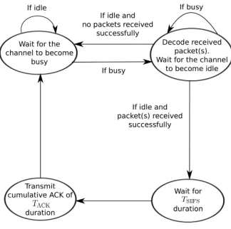
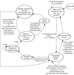
The finite state machines that characterize the behavior of the AP and the nodes in Protocol 2 are shown in Figure 3 and Figure 4, respectively, for saturated traffic conditions.
Remark As in conventional DCF, virtual carrier sensing using the expected duration field in the packet header and the network allocation vector (NAV) can also be implemented in Protocol 2. When the number of ongoing transmissions increases, a node updates its NAV table using the expected duration field of the most recent packet that was transmitted.2 A node can stop sensing the channel once the number of transmissions reaches L or it starts decreasing. Such virtual
2If multiple packet transmissions start at the same time, then the maximum
[image:4.612.337.537.57.198.2]carrier sensing is not as easy in Protocol 1, which allows new packet transmissions to start anytime so long as the total number of ongoing transmissions does not exceedL.
Remark In Protocol 2, channel estimation can be performed at the AP using training symbols in the preambles of each of the received data packets. The reader is referred to the extensive survey of channel estimation issues and techniques in [23] and to the discussion of MPR-specific channel estima-tion issues in [2]. In [24], it was shown that the asynchronous nature of the interference in the MPR MAC protocol even affects the optimal placement of pilots inside a packet. How-ever, modeling and analyzing the effect of imperfect channel estimates is beyond the scope of the paper.
III. ANALYSIS
We now analyze Protocol 2 in saturated traffic conditions in which the transmission queue at each node is always non-empty. Data loss due to packet errors is assumed to be negligible and a transmitted packet is assumed to be received successfully unless it is involved in a collision.
To get compact analytical results, we assume that the transmission duration of a data packet is λ slots, and that the transmission rate is fixed atΩ, as has also been assumed in [18], [19]. Notice that fixed length packets cannot be easily analyzed using the Markovian approach of [16]. Extension to the scenario where the packet lengths are random is discussed at the end of this section. Further, we analyze the L = 2 case, as was also done in [15]. The analysis can be extended to cover the general L ≥ 2 case. However, the expressions become more involved given the larger number of possible transmission scenarios that can occur. Due to space constraints and given the limited additional intuition provided by the general scenario, we do not discuss it in this paper.
As all the nodes use the same backoff parameters, their behaviors are statistically identical. Hence, we make the fol-lowing decoupling approximations, which enable a fixed-point analysis [18], [19]:
1) Each transmitted packet suffers a collision with a prob-ability γ, which is independent of all other nodes and does not depend on the number of its retransmissions. We shall refer to γ as the conditional packet collision probability.
2) Each node attempts a transmission in a slot in which it can transmit with a probabilityβ, which is independent of all other nodes. We shall refer toβas the attempt rate. Node-specific renewal process: Consider a given node, which we henceforth call the tagged node. Let Aj and Bj
respectively denote the number of attempts and total backoff duration (in slots) needed by the tagged node to transmit itsjth packet. Let us consider the process formed by extracting only the times at which the tagged node is in its backoff phase, i.e., it is decrementing its backoff timer. From the first assumption and the fact that the tagged node uses the same backoff param-eters for all its packets, it can be inferred that the sequences (Aj)j≥1, (Bj)j≥1, and (Aj, Bj)j≥1, are all independent and
identically distributed (i.i.d) [19]. Hence, the backoff process of a tagged node is a renewal process with renewal lifetimes
Bj, j ≥ 1, and the renewal epochs are the time instants at
which the node starts the final transmission of itsjth packet. If we consider Aj, j ≥ 1, as the reward gained at the jth
renewal interval, then from the renewal reward theorem [25], we haveβ= E[Aj]
E[Bj], whereE[·]denotes expectation.
System-wide renewal process: Consider the aggregate at-tempt process by all the n nodes. Due to the decoupling assumption, the aggregate attempt process is another renewal process. As shown in Figure 2, the renewal epochs of this process are the instants at which all the nodes start decre-menting their backoff timers. For the rest of the paper, unless mentioned otherwise, the term renewal interval shall refer to the renewal interval of the system-wide renewal process.
Unlike conventional DCF, more than one packet can get transmitted in a renewal interval. We, therefore, first define the following terminology. Forj ∈ {1,2}, a transmitted packet is called thejth packet in a renewal interval if there are already
j−1 ongoing packet transmissions in the channel when its
transmission commences.
Lemma 1: Given that a tagged node transmits in a renewal interval, the probabilityαthat its packet is the first packet in the renewal interval isα= K1(β)
K1(β)+K2(β), whereKi(β)is the
unconditional probability that the tagged node transmits the ith packet in a renewal interval. Further,
K1(β) =
β
1−(1−β)n and (1)
K2(β) =
(n−1)β2(1−β)n−1(1−(1−β)(λ−1)(n−1))
(1−(1−β)n)(1−(1−β)n−1) .
(2)
Proof: The proof is relegated to Appendix A.
Thus, given that a tagged node has transmitted in a renewal interval, the probability that its packet is the second packet in the renewal interval is1−α.
Theorem 1: The conditional packet collision probability,γ, as a function ofβ is given by
γ,Γ(β) =αP1(β) + (1−α)P2(β), (3)
wherePi(β), fori= 1,2, denotes the probability that a packet
suffers a collision given that it is theith transmitted packet in a renewal interval. Further,
P1(β) =
1−(1−β)n−1−(n−1)β(1−β)n−2 1−(1−β)n−1
×1−(1−β)λ(n−1), (4)
P2(β) = 1−(1−β)n−2. (5)
The attempt rate, β, as a function of γ is given
by β , G(γ) = b0+γb1+γ+γ1+γ22b+2+······+γ+γKKb
K, where bk = 1
2 2kCWmin−1
, for0≤k≤K, denotes the mean backoff duration (in slots) before the(k+ 1)th transmission attempt of a packet.
Proof: The proof is relegated to Appendix B.
Hence, combining Lemma 1 and Theorem 1 results in the following fixed-point equation:
Since Γ(G(γ))is a continuous mapping inγfrom the closed set[0,1]to itself, Brouwer’s fixed-point theorem [26] guaran-tees the existence of a fixed-point in the range. Solving this equation numerically yieldsγ. Then, Theorem 1 directly yields β.3
A. Saturation Throughput
Letζdenote the amount of successfully transmitted data at the end of a renewal interval of durationT. From the renewal reward theorem [25], the saturation throughput,S, is given by S = EE[T[ζ]]. We now develop expressions for E[ζ] and E[T]. As shown in Figure 2, a renewal interval of length T starts with an idle period of durationTidle. It is followed by a busy period of length Tbusy, in which one or more packets and a cumulative ACK (if success occurs) are transmitted. The busy period ends once the channel has been idle for the duration TDIFS.
Depending on whether a success or a collision has occurred in the renewal interval, we refer to the busy time period following the idle period as a success period of duration Tsuc or a collision period of durationTcol, respectively. Further, let Tmin
col andTsucmin denote the minimum values of Tcol andTsuc, respectively. It can be seen that Tmin
col = λδ+TDIFS, which occurs when at least three packets of lengthλδare transmitted simultaneously at the end of the idle period. Similarly, we have Tmin
suc =λδ+TSIFS+TACK+TDIFS.
Theorem 2: The expected duration of the renewal interval is E[T] = E[Tidle] +Dcol+Dsuc, where Dcol and Dsuc are the contributions to the average busy period duration from the collision and success events, respectively. Further, E[Tidle] =
1 1−(1−β)n,
Dcol=
1−(1−β)n−nβ(1−β)n−1
1−(1−β)n
−n(n−1)β
2(1−β)n−2
2 (1−(1−β)n)
Tcolmin
+nβ(1−β)
n−1
1−(1−β)n−1−(n−1)β(1−β)n−2 (1−(1−β)n) (1−(1−β)n−1)
×
1−(1−β)(λ−1)(n−1)Tmin
col
+ 1−(1−β)
(λ−1)(n−1) λ−(λ−1)(1−β)n−1
(1−(1−β)n−1) δ
#
, (7)
Dsuc=
n(n−1)β2(1−β)n−2+ 2nβ(1−β)λ(n−1)
2 (1−(1−β)n) T
min
suc
+n(n−1)β
2(1−β)n−1(1−β)n−2
(1−(1−β)n) (1−(1−β)n−1)
×
1−(1−β)(λ−1)(n−1)Tmin
suc
+1−(1−β)
(λ−1)(n−1) λ−(λ−1)(1−β)n−1
(1−(1−β)n−1) δ
#
. (8)
3In our simulations, we have observed that the fixed-point is unique for the
parameters of interest. However, proving uniqueness remains a challenging task.
The expected number of bits transmitted in a renewal interval is given by
E[ζ] = 2λδΩ
n(n−1)β2(1−β)n−2
2 (1−(1−β)n)
+n(n−1)β
2(1−β)n−2
(1−β)n−1−(1−β)λ(n−1) (1−(1−β)n−1)(1−(1−β)n)
!
+λδΩnβ(1−β)
λ(n−1)
1−(1−β)n . (9) Proof: The proof is relegated to Appendix C.
Hence, the expression for the saturation throughput follows directly from Theorem 2.
B. Packet Dropping Probability
A packet is discarded by a node if it suffersK+1collisions. By our first decoupling approximation, a packet collides with a probability γ, which is independent of the number of its retransmission attempts. Consequently, the packet dropping probability is simplyγK+1.
C. Average Head-of-line Packet Delay
The average time spent by a packet in the head-of-queue position before it gets transmitted successfully or dropped after K+1failed transmission attempts is known as the head-of-line
packet delayD.
To evaluate D, we first note that the packet dropping probability, γK+1, is small unless the channel is heavily
congested. Therefore, almost all the packets are eventually successfully transmitted. Hence,D is approximately equal to the average time taken by a node to successfully transmit a packet. Since S is the saturation throughput (in bits) and each packet carries a payload of Ωλδ bits, the number of data packets that are successfully transmitted per unit time is
S
λδΩ. Thus, the number of successfully transmitted data packets
per unit time per node is nλδΩS . Therefore, the average time required to successfully transmit a data packet is D≈nλδΩS .
Remark The fixed-point analysis presented in this section can be extended to handle the scenario where the packet lengths are random variables. It can be shown that the general expressions for K2(β) and P1(β) are obtained by taking
expectations of (2) and (5), respectively, with respect to the distribution of the packet lengths. The expressions for Dcol, Dsuc, andE[ζ]can be derived similarly by summing over all possible realizations of packet lengths of the first and second packets in a renewal interval. All the other expressions remain unchanged.
IV. EFFECT OF IMPERFECT CHANNEL ESTIMATION
The technique can be used if a node is equipped with an array of at least L antennas, which is easily feasible in WLANs today [28], [29].
Let a node be equipped with V ≥ L antennas and let there be U ongoing transmissions in the channel. Also, let yj(t), for j = 1, . . . , V, denote the signal received at the
jth antenna of the node. Noises at different array elements are assumed to be uncorrelated with variance σ2
n. The
cor-relation matrix R associated with the received signal vector
¯
y(t) = [y1(t), . . . , yV(t)]T is defined as R=Ey¯(t)y¯†(t),
where T and † denote transpose and Hermitian transpose, respectively. It can be shown that if U < V then the smallest eigenvalue of Risσ2
n and it has an algebraic multiplicity of
V −U. WhenU ≥V (≥L), Rhas no eigenvalues equal to σ2
n. Thus, by evaluating the multiplicity of the eigenvalue ofR
that is equal to the noise variance, a node can estimate whether the number of ongoing transmissions is 0,1,2, . . . , L−1 or greater than or equal toL.
In practice, sinceRitself is estimated by averaging a finite number of samples taken from the output of the antenna array, its smallest V −U eigenvalues need not be exactly equal to the noise variance. Several papers in the literature, e.g., [30]– [32], solve this problem using approaches based on nested sequence of hypothesis tests, information-theoretic criteria for model selection, and ranking and selection theory.
Imperfect estimation model: A key thing to take away from this discussion is that the presence of noise and channel propagation effects can occasionally make a node incorrectly estimate the number of ongoing transmissions in the channel. This clearly affects the performance of the asynchronous MPR protocols, whose multiple access rules use this estimate. We model imperfect estimation as follows. With probability pi,j,
a node estimates that there j ongoing transmissions while there actually are i.4 We make the following simplifying assumptions: (1) A node makes an error independent of the other nodes. This is justifiable since the channel fades and noise encountered by the different nodes are independent. (2) Once a node estimates the number of transmissions in a slot, its estimate does not change until the transmitters or the number of transmissions actually change. This captures the fact that deep fades are primarily responsible for incorrect estimation. (3) A node perfectly estimates whether the channel is idle or not, i.e., p0,j =pj,0 = 0, for all j ≥1. Similarly,
the odds that a node’s estimate of the number of ongoing transmissions is incorrect by more than one are assumed to be negligible, i.e., pi,j = 0 if |j−i| ≥ 2 for all i ∈ Z+.
We shall also assume that pL−1,L= 0. This intuitive model,
while not general, provides a tractable method to analyze the effect of imperfect estimates, while capturing the essence of the problem.
As before, we analyze below the L = 2 case. The main problem that now arises is that a node can erroneously estimate the number of ongoing transmissions to be one, while there are actually two. It, therefore, will continue to decrement its
4This abstraction presents a refined probabilistic model for the classical
[image:7.612.355.517.59.220.2]hidden nodes problem that arises in conventional DCF, in which the nodes that incorrectly estimate that the number of ongoing transmissions is zero are treated as hidden nodes.
Fig. 3. Protocol 2: Finite state machine for the access point.
timer and eventually it may transmit and cause a collision.
A. Analysis with Imperfect Estimation of Number of Transmit-ters
As in Section III, we use the two classical decoupling approximations. To distinguish from the perfect estimation case, we shall denote the attempt rate by β˜ and the condi-tional packet collision probability byγ. It can be shown that˜
˜
β=G(˜γ), whereG(·) is as defined in Theorem 1.
We now consider the system-wide renewal process. Due to imperfect estimation, a third, and, in general, ajth packet, for j≥3, can be transmitted in a renewal interval. Thejth packet in a renewal interval, forj≥3, is defined as a packet whose transmission commences erroneously whenj−1 nodes have already commenced transmission in the interval.
The erroneous third packet transmission can start, for exam-ple, when the previous two transmissions are still ongoing in the channel. It can also start after the number of transmissions decreases from two to one. This is because the nodes, which had erroneously estimated two transmissions to be one, cannot detect this decrease and continue to decrement their timers. However, the latter scenario is less probable because for it to happen the erroneous node must have a sufficiently large backoff timer value to decrement even after the completion of the first packet’s transmission. In Protocol 2, when the estimation error is small, collisions occur rarely, which makes it less likely for a node to have a large enough contention window. Therefore, we ignore this case and all cases that involve more than one erroneous packet transmissions in a renewal interval.
In order to write compact analytical expressions, we first define the function Θ : Z+ → R+ as Θ(t) = p2,1(1 −
˜
β)t+ 1−p
2,1. It denotes the probability that a node does
not transmit during thetslots in which there are already two ongoing transmissions in the channel.
Lemma 2: Given that a tagged node transmits in a renewal interval, the probabilityα˜i that the packet transmitted by the
tagged node is theith packet in the interval is given by
˜ αi=
˜ Ki( ˜β)
˜
K1( ˜β) + ˜K2( ˜β) + ˜K3( ˜β)
where K˜i( ˜β), fori= 1,2,3, is the unconditional probability
that a tagged node transmits theithpacket in a renewal interval. Furthermore,K˜1( ˜β) =K1( ˜β),K˜2( ˜β) =K2( ˜β), and
˜ K3( ˜β) =
n(n−1) ˜β3(1−β˜)n−2
21−(1−β˜)n λ−2
X
i=0
p2,1(1−β˜)iΘn−3(i)
+(n−1)(n−2) ˜β
3(1−β˜)2n−3
1−(1−β˜)n
×
λ−3
X
i=0 λ−i−3
X
j=0
(1−β˜)i(n−1)+jp2,1Θn−3(j). (11)
Recall that K1(·)andK2(·)are defined in Lemma 1. Proof: The proof is relegated to Appendix D.
Theorem 3: The packet collision probability,γ, in terms of˜ the attempt rate,β˜, is given by
˜
γ,Γ( ˜˜ β) = ˜α1P˜1( ˜β) + ˜α2P˜2( ˜β) + ˜α3P˜3( ˜β), (12)
where α˜i, for i = 1,2,3, are given by Lemma 2. Here,
˜
Pi( ˜β)denotes the probability that a packet suffers a collision
given that it is theith transmitted packet in a renewal interval. Further,
˜
P1( ˜β) =P1( ˜β) + (n−1) ˜β(1−β˜)n−2
×
λ−1
X
i=0
(1−β˜)i(n−1) 1−Θn−2(λ−i−1) , (13)
˜
P2( ˜β) =P2( ˜β) +
(1−(1−β˜)n−1)(1−β˜)n−2
1−(1−β˜)(λ−1)(n−1)
×
λ−2
X
i=0
(1−β˜)i(n−1) 1−Θn−2(λ−i−2) , (14)
and P˜3(β) = 1. Recall that P1(·) and P2(·) are defined in
Theorem 1.
Proof: The proof is relegated to Appendix E.
Hence, by combining (12) and β˜ = G(˜γ), we obtain the desired fixed-point equation in γ. As in ideal channel estimation, the existence of a solution in[0,1]is guaranteed by the Brouwer’s fixed-point theorem [26]. A proof of uniqueness again remains a challenging problem.
B. Throughput
As in Section III-A, it can be shown that the saturation throughput with imperfect estimation is S = EE[T][ζ]. We now evaluate E[T] andE[ζ].
1) Evaluating E[T]: Recall from Lemma 2 that E[T] =
E[Tidle] +Dcol+Dsuc. As before,E[Tidle] = 1 1
−(1−β˜)n. We
now derive expressions forDsuc andDcol.
Evaluating Dsuc: Clearly, Tbusy = Tsucmin when: (i) only one node transmits in the renewal interval, or (ii) exactly two nodes start transmitting simultaneously at the end of the idle period and no other transmissions occur subsequently. Exactly two nodes can do so only when each of the remaining n −2 nodes either does not make an error, or makes an error but does not transmit during the remaining λ−1 slots of the first two packets. The probability of this event is
p2,1(1−β˜)λ−1+ 1−p2,1
n−2
= Θn−2(λ−1). We then
have
PrTbusy=Tsucmin
=nβ˜(1−β˜)
λ(n−1)
1−(1−β˜)n
+
n 2
˜
β2(1−β˜)n−2
1−(1−β˜)n Θ
n−2(λ−1). (15)
The denominator term1−(1−β˜)n arises because of
condi-tioning on the event that the idle period has already ended. Similarly, Tbusy = Tsucmin +kδ when the first and second transmissions in a renewal interval start 1≤k≤λ−1 slots apart and no other transmission occurs subsequently. It can be shown that
PrTsuc=Tsucmin+kδ
=n(n−1) ˜β
2(1−β˜)k(n−1)
1−(1−β˜)n
×(1−β˜)n−2Θn−2(λ−1−k). (16)
Evaluating Dcol: Along similar lines, Tbusy =Tcolmin when at least three amongnnodes start transmitting simultaneously at the end of the idle period. The probability of this event is
PrTbusy=Tcolmin
=1−(1−β˜)
n−nβ˜(1−β˜)n−1
1−(1−β˜)n
−
n 2
˜
β2(1−β˜)n−2
1−(1−β˜)n . (17)
Again, Tbusy = Tcolmin+kδ when: (i) Exactly two of the n nodes transmit the first packet in a renewal interval and the third packet is transmitted erroneously afterkslots by at least one of the remainingn−2nodes, which can be shown to occur with probabilityΘn−2(k−1)−Θn−2(k); or (ii) the first packet
is transmitted by a single node, and afterk slots at least two of the remaining nodes transmit simultaneously; or (iii) the first and second packets are transmittedlslots (1≤l≤k−1) apart, and the third erroneous transmission occurskslots after the first transmission. The probabilities of these events can be calculated in a manner similar to that discussed above. It can be shown that
Pr
Tbusy=Tcolmin+kδ
=
n 2
˜
β2(1−β˜)n−2
1−(1−β˜)n
× Θn−2(k−1)−Θn−2(k)
+n(n−1) ˜β
2(1−β˜)n−2
1−(1−β˜)n
×
"k−1
X
l=1
(1−β˜)l(n−1) Θn−2(k−l−1)−Θn−2(k−l) #
+nβ˜(1−β˜)
k(n−1)
1−(1−β˜)n (1−(1−β˜)
n−1−(n−1) ˜β(1−β˜)n−2).
(18)
Combining the above results yields the expressions for Dsuc andDcol, and, hence,E[T].
2) Evaluating E[ζ]: As in ideal channel estimation, ζ
If the number of sensed transmissions
becomes greater than or
equal to L or decreases
Fig. 4. Protocol 2: Finite state machine for a node under saturated traffic condition.
are successfully transmitted in a renewal interval. The proba-bilities of these events are given in (15) and (16). Hence,
E[ζ] =λδΩnβ˜(1−β˜)
λ(n−1)
1−(1−β˜)n + 2λδΩ
×
n 2
˜
β2(1−β˜)n−2
1−(1−β˜)n Θ
n−2(λ−1)
+ 2λδΩ
λ−1
X
k=1
n(n−1) ˜β2(1−β˜)k(n−1)(1−β˜)n−2
1−(1−β˜)n
×Θn−2(λ−1−k). (19)
V. NUMERICALRESULTS
TABLE I SIMULATION PARAMETERS
Parameter Notation Values
Slot duration δ 20µs
DIFS duration TDIFS 50µs
SIFS duration TSIFS 10µs
Minimum contention window size CWmin 32 Maximum contention window size CWmax 1024 Maximum number of transmissions K+ 1 8
Packet length λ 400slots
ACK duration (with PHY header) TACK 304 + 48(L−1)µs
We now present the results obtained from Monte Carlo simulations that use 50000 samples. An event-driven plat-form written in the C programming language was built for simulating the MPR protocols, and provides an independent verification of the analytical results. The platform implements the finite state machines of the AP and the nodes that are
shown in Figures 3 and 4, respectively. Virtual carrier sensing is not implemented since it does not affect the performance metrics under consideration. The parameter values used in the simulations are listed in Table I. The ACK frame length is increased by 6-bytes for each extra receiver address field to incorporate MPR. We shall vary some of the parameters over a wide range to investigate the sensitivity of the asynchronous MPR MAC protocols to them.
A. Ideal Estimation
[image:9.612.49.301.54.310.2]Figure 5 plots the saturation throughput,S/Ω, as a function of the number of nodes,n, for conventional DCF, Protocol 1, and Protocol 2. The results are shown for different values of L. We observe a good match between the analysis and simulation results for the L = 2 case. We also see that the saturation throughput of Protocol 2 is close toLtimes that of conventional DCF and is10-30%more than that of Protocol 1. Allowing for variable packet lengths in the model could make MPR even more rewarding. Similar results are obtained in Figure 6, which plots the average head-of-line packet delay of the protocols as a function ofnfor variousL. This figure shows that the head-of-line packet delay,D, increases almost linearly with the number of nodes,n. This can be explained by the relation derived in Section III-C and the fact that saturation throughput varies slowly with n. We see that the head-of-line packet delay decreases as L increases. This is because, for larger L, more transmission opportunities are available for a node. This more than compensates for the additional delay caused by more overlapping transmissions in a renewal interval.
To investigate the effect of packet lengths on the perfor-mance of the protocols, we plot in Figure 7 the saturation throughputs of Protocols 1 and 2 as a function of the packet length, λ, for different values of L. We again see that Pro-tocol 2 outperforms ProPro-tocol 1 for a wide range of packet lengths and for all L. We also observe that for large packet lengths, the saturation throughputs of both protocols become almost constant. This can be explained from (7), (8), and (9) as follows: Asλbecomes large the exponential terms containing λ in the expressions forDcol, Dsuc, and E[ζ] become negli-gible. Hence, both E[T] and E[ζ] increase linearly with λ. Thus, their ratio, which is the saturation throughput, becomes almost constant.
We delve into the inner workings of the protocols in Figure 8, which plots the conditional packet collision prob-ability, γ, as a function of n for Protocol 1, Protocol 2 and conventional DCF. As expected,γ increases with n. We observe that the collision probability of Protocol 2 is less than that of Protocol 1 and conventional DCF for all n. Notice that the analysis and simulation results for Protocol 2 match each other well, which validates the fixed-point analysis. As nincreases, the relative error between analysis and simulation decreases. This is in consonance with the results in mean field interaction theory [33].
10 15 20 25 30 35 40 45 50 0
0.5 1 1.5 2 2.5 3 3.5 4 4.5
Number of nodes, n
Normalized saturation throughput, S/
Ω Protocol 2
Protocol 1
L=3 L=5
L=2
[image:10.612.322.544.65.209.2]802.11 DCF basic access
Fig. 5. Saturation throughput as a function of the number of nodes for different values ofL. Analysis results forL= 2for Protocol 2 are shown using circles (◦).
10 15 20 25 30 35 40 45 50
0 50 100 150 200 250
Number of nodes, n
Average head−of−line packet delay (in ms)
Protocol 2 Protocol 1 802.11 DCF
basic access
L=2 L=3
L=5
Fig. 6. Head-of-line average delay per packet as a function of the number of nodes for different values ofL. Analysis results forL= 2for Protocol 2 are shown using circles (◦).
probability decreases asKincreases. This is because for fixed n the collision probabilityγ remains constant. Hence, asK increases, the packet dropping probability γK+1 decreases.
Note that for K ≥4, the packet dropping probability is less than 5% even with 50 nodes.
B. Imperfect Estimation
To investigate the effect of imperfect estimation of number of transmitters, we set p2,1 = p3,2 = . . . =pL,L−1 =p. In
Figure 10, we plot the saturation throughput of Protocol 1, Protocol 2, and the synchronous MPR MAC protocol as a function of p for different values of L. Notice that the saturation throughput of Protocol 2 decreases by only 9% whenpincreases ten-fold from 0.001 to 0.01. Thus, Protocol 2 is robust to estimation errors. Protocol 1 also shows a similar sensitivity levels to the estimation errors. Further, for L= 2, we see a good match between the analysis and simulation results. The saturation throughput of the synchronous protocol does not depend on thepbecause in it a node does not need to estimate the number of ongoing transmissions. Eventually, for large enough p, the saturation throughput of Protocol 2 falls below that of the synchronous protocol. The cross-over point
50 100 150 200 250 300 350 400 450 500 0
0.5 1 1.5 2 2.5 3
Packet length in slot, λ
Normalized saturation throughput, S/
Ω
Protocol 2 Protocol 1 L=2
[image:10.612.60.280.65.209.2]L=4
Fig. 7. Saturation throughput as a function of the packet length for different values ofL. Analysis results forL= 2for Protocol 2 are shown using circles (◦).
10 20 30 40 50 60 70 80 90 100 0
0.1 0.2 0.3 0.4 0.5 0.6
Number of nodes, n
Conditional collision probability,
γ
Protocol 2 (Simulation) Protocol 2 (Analysis) Protocol 1
802.11 DCF (Simulation) 802.11 DCF (Analysis) Proposed
protocol
802.11 DCF
Fig. 8. Conditional packet collision probability as a function of the number of nodes (L= 2).
increases with L.
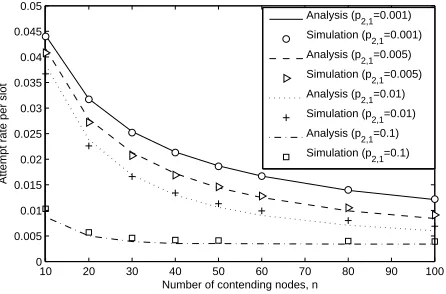
Figure 11 focuses on L = 2 and plots the attempt rate, ˜
β, as a function of n for different values of p2,1. We again
observe a good match between the analytical and simulation results. We see that the attempt rate deceases asp2,1increases,
which happens because the collision probability,γ, increases˜ and the contention window size increases. The increase in the contention window size also explains the minor mismatch between the analytical and simulation results in the above two figures arises for largerpforL= 2.
VI. CONCLUSIONS
[image:10.612.322.544.269.416.2] [image:10.612.60.282.271.419.2]10 20 30 40 50 60 70 80 90 100 0
0.1 0.2 0.3 0.4 0.5 0.6 0.7
Packet dropping probability
Number of nodes, n K=7 (Simulation)
K=7 (Analysis) K=4 (Simulation) K=4 (Analysis) K=2 (Simulation) K=2 (Analysis)
Fig. 9. Packet dropping probability as a function of number of nodes for different settings of maximum number of retransmissions (L= 2).
0 0.02 0.04 0.06 0.08 0.1
0 0.5 1 1.5 2 2.5 3 3.5 4
Estimation error probability, p
Normalized saturation throughput, S/
Ω Protocol 2
Protocol 1
Synchronous MPR protocol
L=2
L=5
[image:11.612.60.285.64.210.2]L=3
Fig. 10. Imperfect estimation scenario: Normalized saturation throughput as a function of estimation error probability for different values ofL. Analysis results forL= 2for Protocol 2 are shown using circles (◦).
protocol. The analysis was generalized to the practical scenario where a node may incorrectly estimate the number of ongoing transmissions. We saw that the asynchronous MPR protocols are quite robust to such errors.
Several interesting avenues for future work exist such as characterizing the non-saturation behavior of the protocol and
10 20 30 40 50 60 70 80 90 100
0 0.005 0.01 0.015 0.02 0.025 0.03 0.035 0.04 0.045 0.05
Number of contending nodes, n
Attempt rate per slot
Analysis (p2,1=0.001)
Simulation (p2,1=0.001)
Analysis (p2,1=0.005)
Simulation (p
2,1=0.005)
Analysis (p2,1=0.01)
Simulation (p2,1=0.01)
Analysis (p2,1=0.1)
Simulation (p
2,1=0.1)
Fig. 11. Imperfect estimation scenario: Attempt rate as a function of the number of nodes (L= 2).
its impact on the performance of higher layers of the protocol stack. While we focused primarily on the single receiver scenario, extension of the protocols to the scenario where multiple transmitter-receiver pairs are simultaneously active, is also an interesting topic for future research. In this case, the ACK handling depends on the physical layer and is affected by antenna systems, channel rank, coding, and network topology.
APPENDIX
A. Proof of Lemma 1
Expression for K1(β): Let the tagged node’s transmission
in slot t (t ≥ 1) of the renewal interval be the first trans-mission in the renewal interval. This occurs with probability (1−β)n(t−1)β, since none of thennodes should have
trans-mitted in the slots 1, . . . , t−1 and the tagged node should transmit in slot t. Hence,K1(β) =Pt=1∞ β(1−β)n(t−1) =
β 1−(1−β)n.
Expression forK2(β): Let the first transmission from a node
other than the tagged node begin in slot t1 of the renewal
interval, where t1 ≥ 1, and let the tagged node transmit
in slot t1 +t2+ 1. Clearly, 0 ≤ t2 ≤ λ−2, since the
Protocol 2 does not permit any node to transmit once the channel becomes idle. The probability of this individual event is(1−β)n(t1−1)(n−1)β(1−β)n−2(1−β)(1−β)(n−1)t2β.
Summing the probabilities over t1 and t2 yields the desired
expression forK2(β).
The expression for α in terms of K1(β) and K2(β) then
follows from Baye’s rule.
B. Proof of Theorem 1
1) Evaluation of Γ(β): The expression for γ follows
di-rectly from the definitions of α, P1(β), and P2(β), and the
law of total probability.
Evaluating P1(β): Let the packet transmitted by a tagged
node be the first packet in a renewal interval. It suffers a collision only if, in any of its λ transmission slots, at least two among the remaining n − 1 nodes transmit. In our protocol, this can happen only when these nodes com-mence transmissions in the same slot. The probability that the first i slots, 0 ≤ i ≤ λ−1, of the transmitted packet are free of collision is (1−β)i(n−1). And, the probability
that two or more nodes transmit in the (i + 1)th slot is 1−(1−β)n−1−(n−1)β(1−β)n−2. Thus, we haveP
1(β) =
Pλ−1
i=0(1−β)i(n−1) 1−(1−β)n−1−(n−1)β(1−β)n−2
, which simplifies to (5).
Evaluating P2(β): If the packet transmitted by a tagged
node is the second packet in a renewal interval, then it suffers a collision only if at least one among the remainingn−2nodes transmits in the same slot as the tagged node. The probability of this event is P2(β) = 1−(1−β)n−2.
2) Evaluation ofG(γ): The expression forG(γ)is based on the node-specific renewal process and follows directly from the equationβ =E[Aj]
[image:11.612.59.281.262.406.2] [image:11.612.59.282.570.717.2]C. Proof of Theorem 2
1) Evaluation of E[T]: A renewal interval of length T
consists of an idle period of duration Tidle followed by a busy period, which is either a collision or a success. Therefore, E[T] = E[Tidle] + Dcol +Dsuc. Here, Dcol =
E[TbusyI[Tcol>0]] and Dsuc = E[TbusyI[Tsuc>0]], where I[ω] denotes an indicator function that equals 1 if ω is true and is 0 otherwise.
Expression for E[Tidle]: A slot is idle with a probability
(1−β)n as none among the n nodes should transmit in it.
Thus, Pr[Tidle> t] = (1−β)nt, fort= 0,1, . . .. Hence,
E[Tidle] =
∞
X
t=0
Pr[Tidle> t] =
∞
X
t=0
(1−β)nt= 1
1−(1−β)n.
(20) Expression for Dcol: Clearly, Tbusy = Tcolmin when at least three nodes commence transmissions simultaneously at the end of the idle period and, thus, collide. This occurs with
proba-bility 1−(1−β)
n−nβ(1−β)n−1−(n
2)β 2(1
−β)n−2
1−(1−β)n . The denominator
is due to the conditioning on the fact that the idle period has already ended and, therefore, at least one node has transmitted. Now,Tbusy=Tcolmin+kδ, for1≤k≤λ−1, when one among n nodes starts transmitting after the idle period, none among the remainingn−1nodes transmit in the nextk−1slots, and then at least two among thesen−1nodes simultaneously com-mence transmission in the next slot. This occurs with proba-bility nβ(1−β)n−
1
(1−β)(k−1)(n−1)(1−(1−β)n−1−(n−1)β(1−β)n−2)
1−(1−β)n .
Combining the terms for the collision events yields Dcol = Pλ−1
k=0Pr
Tbusy=Tcolmin+kδ
(Tcolmin+kδ), which simplifies to (8).
Expression forDsuc: Similarly,Tbusy=Tsucmin when: (i) ex-actly one node transmits in the renewal interval and none of the n−1 nodes transmit thereafter, which occurs with probability
nβ(1−β)n−1
1−(1−β)n (1−β)(n−1)(λ−1), or (ii) exactly two nodes start transmitting simultaneously just after the idle period is over,
which occurs with probability ( n
2)β 2(1
−β)n−2
1−(1−β)n .
Now, Tbusy = Tsucmin +kδ, for 1 ≤ k ≤ λ−1, when exactly one among n nodes starts transmitting after the idle period, during the next k − 1 slots none among the n −1 nodes transmit, and finally exactly one among the n − 1 nodes transmits in the next slot. This happens with probability nβ(1−β)n−1(1−β)1(−k−(11)(−nβ)−n1)(n−1)β(1−β)n−2.
Combining the above success terms, we get
Dsuc = Pλ−
1 k=0Pr
Tbusy=Tsucmin+kδ
(Tmin
suc + kδ), which simplifies to (8).
2) Evaluation of E[ζ]: In a renewal interval, ζ = 0 if a collision occurs, ζ = λδΩ if exactly one node successfully transmits, andζ= 2λδΩwhen exactly two nodes successfully transmit. The probabilities of these events were derived while computing E[T]above. Hence,
E[ζ] = nβ(1−β)
λ(n−1)
1−(1−β)n λδΩ + n 2
β2(1−β)n−2
1−(1−β)n
+
λ−1
X
k=1
n(n−1)β2(1−β)n−2(1−β)k(n−1)
1−(1−β)n
!
2λδΩ. (21)
This upon simplification results in (9).
D. Brief Proof of Lemma 2
The derivations ofK˜1( ˜β)andK˜2( ˜β)are the same as that for
K1(β)andK2(β), respectively, in Appendix A. For evaluating
˜
K3( ˜β), we consider the following two cases that may arise
when the tagged node transmits the third packet in a renewal interval while the previous two transmissions are still ongoing in the channel. As mentioned, the probability of the case where the third packet transmission commences after the first packet transmission has ended is smaller and is neglected.
Case 1: Two nodes, excluding the tagged one, start trans-mitting simultaneously the first two packets in the renewal
interval, which occurs with probability(
n−1
2 )β˜ 2(1
−β)˜n−2
1−(1−β˜)n . Then,
in the subsequent slots, the tagged node and x other nodes (0 ≤ x ≤ n − 3) that have not yet transmitted, er-roneously estimate the number of ongoing transmissions in the channel to be one, which occurs with probability
n−3 x
px+12,1 (1−p2,1)n−3−x. None of thesex+ 1nodes
trans-mits for i slots (0 ≤ i ≤ λ−2) and, finally, the tagged node transmits the third packet in the next slot. This oc-curs with a probability β˜(1−β˜)i(x+1). Hence, the
proba-bility of this case is (
n−1
2 )β˜ 2(1
−β)˜n−2
1−(1−β˜)n
Pn−3
x=0 n−3
x
px+12,1 (1−
p2,1)n−3−xPi=0λ−2β˜(1−β˜)i(x+1). This simplifies to the first
term in the expression for K˜3( ˜β)in Lemma 2.
Case 2: Exactly one among the n nodes excluding the
tagged node transmits the first packet in the renewal interval, say in slot t1, with probability (n−1) ˜β(1−
˜ β)n−1
1−(1−β˜)n . Then in
slot t1 +i+ 1 another node, excluding the tagged node,
transmits the second packet, which occurs with probability (n−2) ˜β(1−β˜)n−2(1−β˜)i(n−1), where 0 ≤ i ≤ λ−3.
Thereafter, the tagged node and x nodes from among the n−3other nodes incorrectly estimate the channel occupancy, which occurs with probability n−x3px+12,1 (1−p2,1)n−3−x. No
transmissions occur forj slots (0≤j≤λ−i−3), and in slot t1+i+ 1 +j+ 1, the tagged node transmits the third packet,
which occurs with probabilityβ˜(1−β˜)j(x+1). Summing over
all the possible values of i, j, and x yields the second term in the expression forK2( ˜β)in Lemma 2.
The expression for α˜i in terms of K˜i( ˜β) in (10) follows
from Baye’s rule.
E. Proof of Theorem 3
The expression forγ˜ follows directly from the law of total probability. Also, if a tagged node erroneously transmits when already there are two ongoing transmissions in the channel, then a collision is inevitable.5 Hence,P˜3( ˜β) = 1.
Expression for P˜1( ˜β): Let the packet transmitted by the
tagged node be the first packet in a renewal interval. The events that contribute to the expression for P˜1( ˜β) are the
same as those that contribute to P1(·)in Appendix B except
that the following additional event can occur due to incorrect estimation: None of the remainingn−1nodes transmit during the first i slots (0≤i≤λ−1) of the packet transmitted by
5This is because, as mentioned, we ignore the unlikely event where the
the tagged node, which occurs with probability(1−β˜)i(n−1).
Then, in slot i + 1, exactly one among the n− 1 nodes transmits, which occurs with a probability(n−1) ˜β(1−β˜)n−2.
Finally, in the remaining λ−i−1 slots of the first packet, at least one of the remainingn−2 nodes erroneously trans-mits, which occurs with probability 1−Θn−2(λ−i−1).
Hence, the probability of this additional collision event is (1 − β˜)i(n−1)(n − 1) ˜β(1 −β˜)n−2 1−Θn−2(λ−i−1)
. Summing it overi and adding it to the expression forP1( ˜β)
yields the expression in (13).
Expression for P˜2( ˜β): The collision event that contributes
to the expression for P2(·) in Appendix B also contributes
to the expression for P˜2( ˜β). Incorrect estimation can lead
to the following additional event, in which the tagged node transmits the second packet in a renewal interval and a collision occurs subsequently due to a third transmission. Say the tagged node transmits in the (i + 2)th slot (0 ≤ i ≤ λ −2) of the first packet transmitted by one node among the other n−1 nodes. Given that the tagged node has transmitted the second packet, the probability of this event is (n−1) ˜β(1−β)˜n−1(1−β)˜i(n−1)β(1˜ −β)˜n−2
(1−(1−β˜)n)K˜2( ˜β) . In the
remain-ing λ −i − 2 slots of the first packet, at least one of the remaining n − 2 nodes erroneously transmits a third packet to cause the collision, which occurs with probability
1−p2,1(1−β˜)λ−i−2+ 1−p2,1
n−2
= 1−Θn−2(λ−i−2).
Summing the probabilities over i and adding them to P2( ˜β)
yields (14).
REFERENCES
[1] IEEE 802.11 Working Group, http://www.ieee802.org/11/index.shtml. [2] L. Tong, Q. Zhao, and G. Mergen, “Multipacket reception in random
access wireless networks: From signal processing to optimal medium access control,” IEEE Commun. Mag., vol. 39, pp. 108–112, Nov. 2001. [3] J. A. Stine, “Exploiting smart antennas in wireless mesh networks using contention access,” IEEE Trans. Wireless Commun., vol. 13, pp. 38–49, Apr. 2006.
[4] F. Shad, T. D. Todd, V. Kezys, and J. Litva, “Dynamic slot allocation (DSA) in indoor SDMA/TDMA using a smart antenna basestation,”
IEEE/ACM Trans. Networking, vol. 9, pp. 69–81, Feb. 2001.
[5] Q. Zhao and L. Tong, “A multiqueue service room MAC protocol for wireless networks with multipacket reception,” IEEE/ACM Trans.
Networking, vol. 11, pp. 125–137, Feb. 2003.
[6] W. L. Huang, K. B. Letaief, and Y. J. Zhang, “Joint channel state based random access and adaptive modulation in wireless LANs with mul-tipacket reception,” IEEE Trans. Wireless Commun., vol. 7, pp. 4185– 4197, Nov. 2008.
[7] L. Tong, V. Naware, and P. Venkitasubramaniam, “Signal processing in random access,” IEEE Signal Proc. Mag., vol. 21, pp. 29–39, Sep. 2004. [8] S. Ghez, S. Verdu, and S. C. Schwartz, “Stability properties of slotted ALOHA with multipacket reception capability,” IEEE Trans. Automat.
Contr., vol. 33, pp. 640–649, Jul. 1988.
[9] S. Ghez, S. Verdu, and S. C. Schwartz, “Optimal decentralized control in the random-access multipacket channel,” IEEE Trans. Automat. Contr., vol. 34, pp. 1153–1163, Nov. 1989.
[10] V. Naware, G. Mergen, and L. Tong, “Stability and delay of finite user slotted ALOHA with multipacket reception,” IEEE Trans. Inform.
Theory, vol. 51, pp. 2636–2656, Jul. 2005.
[11] Q. Zhao and L. Tong, “A dynamic queue protocol for multiaccess wireless networks with multipacket reception,” IEEE Trans. Wireless
Commun., vol. 3, pp. 2221–2231, Jun. 2004.
[12] D. S. Chan and T. Berger, “Performance and cross-layer design of CSMA for wireless networks with multipacket reception,” in Proc. IEEE
Asilomar Conf. Signals, Syst., Computers (ACSSC), vol. 2, pp. 1917–
1921, Nov. 2004.
[13] R. H. Gau, “Modeling the slotted nonpersistent CSMA protocol for wire-less access networks with multiple packet reception,” IEEE Commun.
Lett., vol. 13, pp. 797–799, Oct. 2009.
[14] P. X. Zheng, Y. J. Zhang, and S. C. Liew, “Multipacket reception in wireless local area networks,” in Proc. ICC, pp. 3670–3675, Jun. 2006. [15] S. Barghi, H. Jafarkhani, and H. Yosefi’zadeh, “MIMO-assisted MPR-aware MAC design for asynchronous WLANs,” IEEE/ACM Trans.
Networking, vol. 19, pp. 1652–1665, Dec. 2011.
[16] F. Babich and M. Comisso, “Theoretical analysis of asynchronous multi-packet reception in 802.11 networks,” IEEE Trans. Commun., vol. 58, pp. 1782–1794, Jun. 2010.
[17] F. Babich, M. Comisso, and A. Dorni, “Multi-packet communication in 802.11 networks: A MAC/PHY backward compatible solution,” in Proc.
Globecom, pp. 1–5, Dec. 2011.
[18] G. Bianchi, “Performance analysis of the IEEE 802.11 distributed coordination function,” IEEE J. Sel. Areas Commun., vol. 18, pp. 535– 547, Mar. 2000.
[19] A. Kumar, E. Altman, D. Miorandi, and M. Goyal, “New insights from a fixed point analysis of single cell IEEE 802.11 WLANs,” IEEE/ACM
Trans. Networking, vol. 15, pp. 588–601, Jun. 2007.
[20] A. Kumar and D. Patil, “Stability and throughput analysis of unslot-ted CDMA-ALOHA with finite number of users and code sharing,”
Telecommun, Syst., vol. 8, pp. 257–275, 1997.
[21] T. Issariyakul, D. Niyato, E. Hossain, and A. S. Alfa, “Exact distribution of access delay in IEEE 802.11 DCF MAC,” in Proc. Globecom, pp. 25– 38, Dec. 2005.
[22] M. M. Carvalho and J. J. Garcia-Luna-Aceves, “Delay analysis of IEEE 802.11 in single-hop networks,” in Proc. IEEE Intl. Conf. Network
Protocols, pp. 146–155, Nov. 2003.
[23] M. Jiang and L. Hanzo, “Multiuser MIMO-OFDM for next-generation wireless systems,” Proc. IEEE, vol. 95, pp. 1430–1469, Jul. 2007. [24] C. Budianu and L. Tong, “Channel estimation under asynchronous
packet interference,” IEEE Trans. Signal Process., vol. 53, pp. 333–345, Jan. 2005.
[25] R. W. Wolff, Stochastic Modeling and the Theory of Queues. Prentice Hall, 1989.
[26] M. A. Khamsi and W. A. Kirk, An Introduction to Metric Spaces and
Fixed Point Theory. John Wiley, 2001.
[27] L. C. Godara, “Application of antenna arrays to mobile communications– part II: Beam forming and direction-of-arrival considerations,” Proc.
IEEE, vol. 85, pp. 1193–1245, Aug. 1997.
[28] T. Kaiser, “When will smart antennas be ready for the market? Part I,”
IEEE Sig. Proc. Mag., vol. 22, pp. 87–92, Mar. 2005.
[29] M. Z. Siam and M. Krunz, “An overview of MIMO-oriented channel access in wireless networks,” IEEE Wireless Commun., vol. 15, pp. 63– 69, Feb. 2008.
[30] D. N. Lawley, “Tests of significance of the latent roots of the covariance and correlation matrices,” Biometrika, vol. 43, pp. 128–136, Jun. 1956. [31] M. Wax and T. Kailath, “Detection of signals by information theoretic criteria,” IEEE Trans. Acoust., Speech, Signal Process., vol. 33, pp. 387– 392, Apr. 1985.
[32] P. Chen, M. Wicks, and R. Adve, “Development of a procedure for detecting the number of signals in a radar measurement,” IEE Proc.
Radar, Sonar Navig., vol. 148, pp. 219–226, Aug. 2001.
[33] M. Benaim and J. Y. L. Boudec, “A class of mean field interaction models for computer and communication systems,” Perform. Eval., vol. 20, pp. 243–302, Nov. 2008.
PLACE PHOTO HERE
PLACE PHOTO HERE
Neelesh B. Mehta (S’98-M’01-SM’06) received his Bachelor of Technology degree in Electronics and Communications Eng. from the Indian Institute of Technology (IIT), Madras in 1996, and his M.S. and Ph.D. degrees in Electrical Eng. from the California Institute of Technology, Pasadena, CA, USA in 1997 and 2001, respectively. He is now an Associate Pro-fessor in the Dept. of Electrical Communication Eng. at the Indian Institute of Science (IISc), Bangalore, India. Prior to joining IISc in 2007, he was a research scientist in AT&T Laboratories, NJ, USA, Broadcom Corp., NJ, USA, and Mitsubishi Electric Research Laboratories (MERL), MA, USA from 2001 to 2007.
His research includes work on link adaptation, multiple access protocols, cellular system design, MIMO and antenna selection, cooperative communi-cations, energy harvesting networks, and cognitive radio. He was also actively involved in the Radio Access Network (RAN1) standardization activities in 3GPP from 2003 to 2007. He was a TPC co-chair for tracks/symposia in ICC 2013, WISARD 2010 & 2011, NCC 2011, VTC 2009 (Fall), and Chinacom 2008. He has co-authored 35 IEEE transactions papers, 60+ conference papers, and three book chapters, and is a co-inventor in 20 issued US patents. He is an Editor of IEEE Wireless Communications Letters and the Journal for Communications and Networks, and currently serves as the Director of Conference Publications in the Board of Governors of the IEEE Communications Society.
PLACE PHOTO HERE