http://wrap.warwick.ac.uk
Original citation:
Docherty, Stephanie Y., Borg, Matthew K., Lockerby, Duncan A. and Reese, Jason M..
(2014) Multiscale simulation of heat transfer in a rarefied gas. International Journal of
Heat and Fluid Flow . ISSN 0142-727X
Permanent WRAP url:
http://wrap.warwick.ac.uk/61995
Copyright and reuse:
The Warwick Research Archive Portal (WRAP) makes this work of researchers of the
University of Warwick available open access under the following conditions.
This article is made available under the Creative Commons Attribution 3.0 (CC BY 3.0)
license and may be reused according to the conditions of the license. For more details
see:
http://creativecommons.org/licenses/by/3.0/
A note on versions:
The version presented in WRAP is the published version, or, version of record, and may
be cited as it appears here.
Multiscale simulation of heat transfer in a rarefied gas
Stephanie Y. Docherty
a,⇑, Matthew K. Borg
a, Duncan A. Lockerby
b, Jason M. Reese
ca
Department of Mechanical & Aerospace Engineering, University of Strathclyde, Glasgow G1 1XJ, UK b
School of Engineering, University of Warwick, Coventry CV4 7AL, UK c
School of Engineering, University of Edinburgh, Edinburgh EH9 3JL, UK
a r t i c l e
i n f o
Article history:
Received 23 December 2013 Received in revised form 30 April 2014 Accepted 7 June 2014
Available online xxxx
Keywords:
Heterogeneous multiscale simulation Hybrid methods
DSMC
Heat flux coupling Rarefied gas dynamics
a b s t r a c t
We present a new hybrid method for dilute gas flows that couples a continuum-fluid description to the direct simulation Monte Carlo (DSMC) technique. Instead of using a domain-decomposition framework, we adopt a heterogeneous approach with micro resolution that can capture non-equilibrium or non-con-tinuum fluid behaviour both close to bounding walls and in the bulk. A connon-con-tinuum-fluid model is applied across the entire domain, while DSMC is applied in spatially-distributed micro regions. Using a field-wise coupling approach, each micro element provides a local correction to a continuum sub-region, the dimen-sions of which are identical to the micro element itself. Interpolating this local correction between the micro elements then produces a correction that can be applied over the entire continuum domain. Key advantages of this method include its suitability for flow problems with varying degrees of scale separa-tion, and that the location of the micro elements is not restricted to the nodes of the computational mesh. Also, the size of the micro elements adapts dynamically with the local molecular mean free path. We demonstrate the method on heat transfer problems in dilute gas flows, where the coupling is performed through the computed heat fluxes. Our test case is micro Fourier flow over a range of rarefaction and tem-perature conditions: this case is simple enough to enable validation against a pure DSMC simulation, and our results show that the hybrid method can deal with both missing boundary and constitutive information.
Ó2014 The Authors. Published by Elsevier Inc. This is an open access article under the CC BY license (http:// creativecommons.org/licenses/by/3.0/).
1. Introduction
While the conventional hydrodynamic equations are generally excellent for modelling the majority of fluid flow problems, the presence of localised regions of non-continuum or non-equilibrium flow can result in some degree of inaccuracy. Such regions appear when the flow is far from local thermodynamic equilibrium, for example, when there are large gradients in fluid properties, or when surface effects become dominant. Although molecular simu-lation tools can provide an accurate modelling alternative in these cases, they are usually much too computationally expensive for resolving engineering spatial and temporal scales. Multiscale methodologies that exploit ‘scale separation’ have therefore been developed over the past decade. Scale separation occurs when the variation of hydrodynamic properties across small regions of space or periods of time is only very loosely coupled with the flow behaviour on a much larger spatial or temporal scale.
Often referred to as ‘hybrids’, these multiscale methods com-bine continuum and molecular descriptions of the flow. A
tradi-tional continuum description is employed in macro flow regions, and a molecular treatment is applied in small-scale micro or nano regions. Essentially, the aim is to combine the best of both solvers: the computational efficiency associated with continuum methods, and the detail and accuracy of molecular techniques.
In the literature, two different hybrid frameworks have emerged for fluid flows: (a) the domain-decomposition technique, and (b) the Heterogeneous Multiscale Method (HMM). For liquids, molecular dynamics (MD) is the appropriate molecular simulation tool. This deterministic method is, however, inefficient for dilute gas flows, and the direct simulation Monte Carlo (DSMC) method (Bird, 1998) can instead provide a coarse-grained molecular description. Founded on the kinetic theory of dilute gases, DSMC reduces computational expense by adopting a stochastic approxi-mation for the molecular collision process.
Typically, thermodynamic non-equilibrium effects occur in the vicinity of bounding surfaces or other interfaces. Recognising this behaviour, domain-decomposition has become the most popular
hybrid framework for both liquids (O’Connell and Thompson,
1995; Hadjiconstantinou and Patera, 1997; Flekkøy et al., 2000; Delgado-Buscalioni and Coveney, 2003; Werder et al., 2005) and
dilute gases (Wadsworth and Erwin, 1990; Hash and Hassan,
http://dx.doi.org/10.1016/j.ijheatfluidflow.2014.06.003 0142-727X/Ó2014 The Authors. Published by Elsevier Inc.
This is an open access article under the CC BY license (http://creativecommons.org/licenses/by/3.0/). ⇑ Corresponding author. Tel.: +44 7860 366 574.
E-mail address:stephanie.docherty@strath.ac.uk(S.Y. Docherty).
Contents lists available atScienceDirect
International Journal of Heat and Fluid Flow
j o u r n a l h o m e p a g e : w w w . e l s e v i e r . c o m / l o c a t e / i j h f f
1996; Garcia et al., 1999; Aktas and Aluru, 2002; Roveda et al., 1998; Sun et al., 2004; Sun and Boyd, 2002; Wijesinghe et al., 2004; Wu et al., 2006; Schwartzentruber et al., 2007; Lian et al., 2008). In this method, the simulation domain is partitioned — a molecular solver is applied in the regions closest to the surfaces, while a conventional continuum fluid solver is implemented in the remainder. These micro and macro sub-domains are indepen-dent but communicate through an overlap region that enables mutual coupling. This coupling is typically established by matching fluxes of fluid mass, momentum, and energy, or by matching state properties. However, despite its popularity, a fundamental disad-vantage of this micro–macro decomposition approach is that com-putational efficiency can only be increased above that of a full molecular simulation when non-continuum flow is confined to ‘near-wall’ regions. In highly non-equilibrium flows, or when the temperature dependence of fluid properties such as dynamic vis-cosity or thermal conductivity is not knowna priori(for example, in unusual chemically-reacting gas mixtures), the traditional fluid constitutive relations may be inaccurate in the bulk of the domain. Domain-decomposition techniques are also inappropriate for simulating flow through micro or nanoscale geometries that have a high aspect ratio, e.g. one dimension of the geometry is orders of magnitude larger than another. This class of flow presents a challenge as it requires simultaneous solution of the microscopic processes occurring over the smallest dimension and the macro-scopic processes occurring over the largest dimension, and is often too computationally intensive for a full molecular approach. Such flows are generally beyond the reach of domain-decomposition as the majority (or perhaps all) of the flowfield can be considered ‘near-wall’.
The less-common HMM framework overcomes the limitations
of domain-decomposition by adopting a micro-resolution
approach that can be employed anywhere in the domain — near bounding surfaces, or in the bulk flow. In this case, a continuum model is applied across the entire flow field, and the molecular sol-ver is applied in spatially-distributed micro regions. These micro regions provide the missing data that is required for closure of the local continuum model, either in the form of unknown bound-ary conditions, or unknown constitutive information. Existing HMM studies in the literature are mainly for liquid flows, using
MD as the molecular solver (Ren and E, 2005; Yasuda and
Yamamoto, 2008; Asproulis et al., 2012; Borg et al., 2013). Gener-ally, these studies consider flow problems where momentum transport is dominant and the transfer of heat is negligible. Cou-pling is therefore based on momentum: velocity fields or strain-rates are prescribed in each micro region, and the resultant stress is used to apply a correction back into the hydrodynamic
momen-tum equation (Ren and E, 2005; Yasuda and Yamamoto, 2008).
Each HMM micro region supplies information to a computational
node on the continuum mesh. Thispoint-wise couplingapproach
(Asproulis et al., 2012) is ideal when there is a large degree of spa-tial scale separation in the system, providing significant computa-tional savings over a pure molecular simulation. However, in flow problems with smaller, or mixed, degrees of spatial scale separa-tion, the molecular resolution required can result in the micro ele-ments overlapping, making HMM more expensive and less accurate than a pure molecular treatment.
Despite its advantages over domain-decomposition techniques, there has been little development of HMM-type hybrids that use
DSMC as the molecular treatment. In 2010,Kessler et al. (2010)
proposed the Coupled Multiscale Multiphysics Method (CM3) that
couples both momentum and heat transfer, with DSMC providing corrections to both the hydrodynamic momentum and energy equations. This method was, however, developed to simulate tran-sient flows where a time-accurate solution is sought, and so any computational advantage over a full DSMC simulation is achieved
only through decoupling of the time scales; the length scales remain fully coupled, with both the continuum description and DSMC employed over the same region of space. More recently,
Patronis et al. (2013)adapted the Internal-flow Multiscale Method (IMM) to simulate dilute gas flows with DSMC. Originally
devel-oped byBorg et al. (2013)for liquid flows, IMM adopts a
frame-work similar to HMM but is tailored to model flows in high-aspect-ratio channels. Although large computational savings are presented, this method is tailored specifically to deal with cases where the length scale in the direction of flow is significantly larger than the length scales transverse to the flow direction.
In this paper we propose a new form of the HMM technique, with DSMC providing the molecular description. We adopt the field
wise coupling (HMM–FWC) approach developed by Borg et al.
(2013)for liquid flows: rather than supplying a correction to a node on the continuum mesh, each micro element instead corrects a continuum sub-region, the spatial dimensions of which are iden-tical to those of the micro element itself. This means that, unlike point wise coupling, HMM–FWC is suitable for dealing with flow problems with varying degrees of spatial scale separation. Also, the location of each micro element is not restricted to the nodes of the computational mesh: both the position and size of the micro elements can be optimised for each problem, independently of the continuum mesh.
Our method is designed to cope with inaccuracy in the tradi-tional flow boundary conditions and/or constitutive relations, and is therefore able to deal with problems that are beyond the reach of domain-decomposition. This includes problems where the fluid behaviour is unknown in the bulk, i.e. the traditional con-stitutive relations fail due to non-equilibrium effects (for example, in the wake of a re-entry vehicle), or the transport properties are unknown (for example, in unusual gas mixtures). The method is also suitable for simulating high aspect ratio geometries. While the IMM is designed to simulate problems where the largest length scale is in the flow direction, our new method has no such restric-tion and so provides a more general approach. It could therefore be useful when the largest length scale is transverse to the flow direc-tion; for example, the flow through microscale cracks that can appear in valves.
The form of the method we present in this paper is tailored to model heat transfer problems in dilute gas flows. As a starting point we consider problems in which the gas is essentially motion-less, with large applied temperature gradients placing the focus on heat transfer. With negligible transport of momentum, our cou-pling is performed through the heat flux: we impose the local tem-perature fields on the micro elements and measure the consequent heat flux from the relaxed DSMC particle ensembles. A suitable correction is then applied to the hydrodynamic conservation of energy equation. (Full coupling of mass, momentum, and heat transfer is a subject for future work.)
The level of translational non-equilibrium in a rarefied gas is
generally characterized by the Knudsen number Kn, defined as
the ratio of the gas molecular mean free pathkto a characteristic system dimension L. Typically, the traditional ‘no-temperature-jump’ boundary condition at a bounding surface (wall) is only valid whenKn<0:001; the flow is then in thermodynamic equilibrium as the frequency of both intermolecular and molecule-wall colli-sions is very high. AsKnincreases above 0:001, this collision fre-quency decreases, resulting in a temperature discontinuity between the wall and its adjacent gas. For lowKn, the conventional conservation equations can be extended to account for this by employing von Smoluchowski temperature-jump boundary condi-tions (von Smoluchowski, 1898). However, asKnincreases, mole-cule-wall collisions become more frequent than intermolecular collisions and the thermal Knudsen layer becomes significant. This is essentially a region of non-equilibrium that extends from the
wall into the domain, with its thickness determined by the degree of rarefaction. In this layer, the gas behaviour deviates from the conventional linear heat-flux/temperature-gradient constitutive relation. Even with the use of temperature-jump boundary condi-tions, the conventional hydrodynamic equations cannot model this phenomenon. Our hybrid method, however, aims to capture both the temperature-jump and the thermal Knudsen layer at a lower computational cost than a full-domain DSMC treatment.
This paper is organised as follows. In Section2, we discuss the macro and micro descriptions of the flow. We then present the general three-dimensional form of our multiscale coupling frame-work and its iterative algorithm. For simplicity, one-dimensional heat transfer is considered when validating the method in
Sec-tion 3, with results compared with pure DSMC simulations at
equivalent conditions. In Section4we draw our conclusions.
2. Multiscale methodology
2.1. Continuum description
For simplicity in this paper we restrict our attention to steady-state problems where the gas remains stationary, i.e. it has no streaming velocity. With negligible transport of mass and momen-tum, the continuum description is based on the conservation of energy,
r
q¼0; ð1Þwhereqis the heat flux vector. To close this equation, a suitable constitutive relation is required. For conventional gas flows, the tra-ditional Navier–Stokes-Fourier (NSF) constitutive relations are accurate and so Fourier’s law can be used, i.e.
q¼
j
r
T; ð2Þwhere
j
is the thermal conductivity of the gas. The energy equation then reads,r
ðj
r
TÞ ¼0: ð3ÞAssuming no-temperature-jump boundary conditions, solution of this conventional energy equation will produce a continuum NSF temperature field TNSF. This field is taken as an initial condition
for our hybrid method, and provides a starting point from which the coupling framework iterates towards the correct temperature field.
While Eq.(2)is valid for typical flow problems, it fails in certain flow conditions, for instance, in flows of complex fluids or in ditions of thermodynamic non-equilibrium. Inaccuracy in the con-ventional constitutive model can therefore be quantified by a heat-flux-correction fieldU, so that
q¼
j
r
TþU: ð4ÞThe flux-correction field incorporates not only the departure of the gas state from equilibrium, but also any additional inaccuracy due to the assumed thermal conductivity model. Using this relation to close Eq.(1)results in a ‘flux-corrected’ energy equation,
r
ðj
r
TÞr
U¼0: ð5ÞThe general strategy of our heterogeneous hybrid approach is there-fore as follows. Across each individual micro element, the heat flux and temperature fields are measured. The flux-correction field across each element is then computed using Eq.(4). By
interpolat-ing between all micro elements, the full flux-correction field U
across the entire flowfield is approximated. With this, and the boundary information obtained from micro simulations located at the bounding walls, an appropriate continuum method (e.g. finite difference, finite element, or finite volume) can be used to solve Eq.(5). This produces a flux-corrected continuum temperature field
TUacross the domain. With continuing iterations, this temperature field should converge towards that which would be obtained from a full molecular simulation of the problem.
2.2. DSMC technique
As we focus on heat transfer in dilute gases, we use DSMC as our molecular model in the micro elements. DSMC has become the dominant method for simulating dilute gas flows that lie in the continuum-transition regime. The fundamental concept is to track a large number of numerical particles, storing their position, veloc-ity, and internal state as they move through a computational mesh. During a simulation, the particles collide with each other and with bounding surfaces while maintaining conservation of mass, momentum, and energy. A major advantage of the method is that two key approximations significantly reduce computational expense: (a) each simulated particle typically represents a large number of real gas molecules, and (b) molecular motion and inter-molecular collisions can be decoupled over small time intervals. Particle movements are computed deterministically, while inter-particle collisions are treated statistically within numerical mesh cells.
Using expressions provided byBird (1998), local hydrodynamic properties (including the temperature and the heat flux) can be recovered in DSMC by averaging microscopic data over all of the particles in each cell. However, the inherent statistical scatter asso-ciated with the method means that a large number of independent samples are usually required to capture smooth fields, particularly for low speed flows. Therefore, time averaging is typically used for steady state problems, while ensemble averaging is used for tran-sient flow problems. For continuum-molecular hybrids, the smoothing of statistical fluctuations is particularly important as the transfer of noisy data to the continuum fluid description may result in instability. Consequently, each DSMC simulation in this paper is performed in two stages: a transient period enables the simulation to reach steady-state, and then a longer averaging per-iod reduces the statistical scatter in the measured hydrodynamic properties.
The open-source C++ toolboxOpenFOAM (2013)incorporates a
DSMC solver, dsmcFoam, which has been validated for various benchmark cases, including hypersonic and microchannel flows (Scanlon et al., 2010; Arlemark et al., 2012; White et al., 2013). This is used to perform all of the micro and full-scale DSMC simulations in this paper.
2.3. Coupling framework
In our framework, the continuum description is applied across the entire macro domain, while DSMC is performed in dispersed micro elements (the arrangement of which depends on the flow problem being investigated). As discussed in the Introduction, we propose a new strategy to achieve two-way coupling between these domains. The underlying methodology presented here is general and may be applied to 1D, 2D, or 3D problems.
2.3.1. Macro-to-micro coupling: constraint of the micro elements
It is crucial that the flux-correction information is extracted from DSMC elements in which the gas state is properly representa-tive of the local conditions in the macro domain. There is, however, a fundamental problem in creating such elements: the particle dis-tribution required at the boundaries of the element cannot be extracted directly from the macroscopic continuum flowfield. For this reason, macro-to-micro coupling remains a challenge in mul-tiscale hybrids. In our method, we circumvent this problem by not imposing an exact particle distribution at these boundaries;
instead, we allow the distribution to be dictated by the macro-scopic continuum fields alone.
A natural evolution to the correct particle distribution and mac-roscopic state at the boundaries of an element is possible by estab-lishing an artificial relaxation region (zone) around the element. It is not essential that the gas state in these relaxation zones accu-rately represent the conditions in the corresponding macro domain; their sole purpose is to develop the boundary conditions for the core of the element. Sampling of property fields is per-formed only in the core region, which we refer to as the ‘sampling zone’.
Suitable boundary conditions to the sampling zone are gener-ated by enforcing the continuum variation of macroscopic proper-ties (i.e. in our case, the continuum temperature field) across the surrounding relaxation zone. This is done by implementing particle controllers (Borg et al., 2010). A particle distribution does, how-ever, need to be applied at the outer boundaries of the relaxation zone. This imposed distribution introduces error in the local distri-bution close to these boundaries, and so it is important that the particle state within the sampling zone is sufficiently independent of this introduced error. If the relaxation zone is large enough (i.e. several molecular mean free paths), the form of the imposed distri-bution1is irrelevant — its effect will decay through the zone as the
particle state gradually relaxes through interparticle collisions.
Com-plete relaxation needs to occur over the extent of the relaxation zone such that the particle distribution in the sampling zone is dictated solely by the applied continuum state. Once the hybrid method has converged, the artificiality of the outer relaxation zone dissolves seamlessly into the true particle distribution and fluid state in the inner sampling zone.
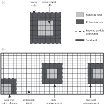
Fig. 1a shows a typical ‘bulk’ micro element in 2D. Similarly,
Fig. 1b shows an example computational domain set-up for a 2D problem, including both bulk and ‘near-wall’ micro elements. In summary, the sampling zone in a micro DSMC element is sur-rounded by the relaxation zone over which the local continuum fields are imposed, and a chosen particle distribution is applied at the outer boundaries. However, in order to capture regions of non-equilibrium that often appear at solid bounding surfaces or walls, the sampling zone in a near-wall micro element must be adjacent to the wall itself. The arrangement of the micro elements is clearly crucial to the overall accuracy of our method, and the appropriate arrangement will vary from problem to problem.
To impose the local continuum temperature field, we divide the relaxation zone in each micro element into a grid of control cells as shown inFig. 1. Using particle controllers (Borg et al., 2010), the appropriate temperature is then set in each control cell to create the desired temperature variation. Similarly, the sampling zone of each micro element is divided into a grid of measurement cells. We then extract the averaged hydrodynamic properties from each measurement cell, enabling us to capture the property fields across the entire sampling zone. Boundary information is also obtained from these measurement cells: we extract the temperature of the gas in contact with the wall from the wall-adjacent cell faces.
Relaxation zone
Sampling zone
Imposed particle
distribution
Solid wall
near-wall
micro element
near-wall
micro element
bulk
micro element
continuum
mesh
control
cells
measurement
cells
(a)
[image:5.595.119.463.66.409.2](b)
Fig. 1.Schematic of (a) a 2D bulk micro element showing the control and measurement cells, and (b) an example computational domain for a 2D problem. The control and measurement cells are independent of the DSMC computational cells, and can also be independent of the continuum mesh.
1
We implement local Maxwellian distributions at the outer edges of the relaxation zones for simplicity. Chapman–Enskog distributions could also be used; as these include perturbations from equilibrium, they may reduce the required size of the relaxation zones.
Essentially, these measurement and control cells form a mea-surement/control mesh that is completely independent of the com-putational mesh used by DSMC itself. This has the benefit of enabling us to define the resolution of the macroscopic fields that we both extract and impose, and to control the noise in our mea-surements, without affecting the accuracy of the DSMC calcula-tions (i.e. the particle collision rate). InFig. 1, the measurement and control cells are shown to have the same dimensions, but this does not have to be the case. Also, inFig. 1b, the measurement and control cells are shown to be collocated with the computational cells of the continuum mesh; although this simplifies the transfer of data between the micro elements and the continuum descrip-tion, it is only for convenience and is not essential. If these cells are not collocated, we simply interpolate between the meshes.
2.3.2. Micro-to-macro coupling: correcting the continuum description
The ease in converting microscopic particle information into macroscopic fields means that, generally, micro-to-macro coupling is less problematic than macro-to-micro coupling. Based on the property fields extracted from the DSMC solver, a suitable correc-tion can be applied to the continuum descripcorrec-tion. In our coupling strategy, this correction is in the form of a heat-flux-correction fieldU, as discussed in Section2.1.
In our DSMC simulations, the average translational temperature (for a single species gas) in each measurement cell is computed from,
Ttr¼ 1 3kB
mc02¼ 1
3kB
m c02
x þc0y2þc0z2
; ð6Þ
wherekBis the Boltzmann constant,mis the molecular mass and
c0
x; c0y, andc0zare thex; y, andzcomponents of the thermal velocity
vectorc0. Assuming the gas has no vibrational energy, the average
heat fluxqin each measurement cell is obtained from,
qqj¼
1 2mnc0
2c0
jþn
e
rotc0j; ð7Þwherejrepresents thex; y, andzcomponents,nis the number den-sity of the gas, and
e
rotis the rotational energy of a single molecule.Note that we consider monatomic gas flows in this paper, and so
e
rot¼0 and the macroscopic temperature T¼Ttr. By computingthe average macroscopic temperature and heat flux in each mea-surement cell, we capture the temperature and heat flux fields across the sampling zone of each micro element. Substituted into Eq.(4), these then provide the flux-correction field across this zone. However, the continuum description is applied across the full
sim-ulation domain, and so Eq.(5) requires the flux-correction field
across the full domain. This field can be approximated using appro-priate interpolation between all the sampling zones.
This hybrid methodology not only corrects for inaccurate con-stitutive information, but also provides missing boundary informa-tion, i.e. the temperature jump. In each near-wall sampling zone, we measure the temperature of the gas in contact with the wall by summing over all particles that strike the surface (Lofthouse, 2008), i.e.
Tgas;wall¼ m
3kB
P
½ðm=jcnjÞðkckÞ Pðm=jcnjÞU2slip
P
ð1=jcnjÞ
; ð8Þ
wherecnis the particle velocity normal to the wall,ctis the particle
velocity tangential to the wall,kckis the velocity magnitude, and
Uslipis the slip velocity which, with zero wall velocity, is given by
Uslip¼
P½ðm=jc
njÞct
Pðm=jc
njÞ
: ð9Þ
We then interpolate this boundary gas temperature between the near-wall sampling zones to produce an estimate of the gas temper-ature at all bounding surfaces.
Using this boundary information and the full flux-correction fieldU, solution of Eq.(5)then produces a new (flux-corrected) temperature fieldTUacross the whole domain. The process is then repeated untilTUrelaxes to a solution that is close to that obtained from a full DSMC simulation.
2.4. Iterative algorithm
The general iterative coupling procedure of this method is:
(0) Assuming no-temperature-jump at bounding surfaces, solve
the conventional energy equation (3) to obtain an initial
estimate for the temperature field across the entire simula-tion domain,TNSF.
(1) Constrain each micro element by applying boundary conditions:
(a) Using particle control in each control cell, enforce the local continuum temperature variation throughout the relaxation zone.
(b) At the outer boundaries of the relaxation zone, impose Maxwellian particle distributions at the local continuum temperature.
(2) Execute DSMC in each micro element as described in Sec-tion2.2. When steady-state is reached, perform averaging of properties in all measurement cells across the sampling zone of each element. Extract the temperature and the heat flux values from each of these cells. Also, from each wall-adjacent measurement cell face, extract the temperature of the gas at the wall surface.
(3) Compute the flux-correction in each measurement cell using the temperature and heat flux values extracted from that cell in the flux-corrected constitutive relation(4). From this, obtain the flux-correction field across each sampling zone. (4) Carry out appropriate interpolations between sampling
zones to approximate the flux-correction fieldUacross the
full simulation domain. Similarly, perform appropriate inter-polations between near-wall sampling zones to obtain the gas temperature at all bounding walls.
(5) Using the boundary gas temperature information and the full flux-correction field, solve the flux-corrected energy equation(5)across the full domain to obtain a new flux-cor-rected temperature fieldTU.
(6) Repeat from Step (1) untilTUdoes not change between iter-ations to within a user-defined tolerance.
3. Validation: one-dimensional Fourier flow
A simple test case is chosen in order to assess the performance of the coupling method, and to easily validate it against a full DSMC simulation. We demonstrate the method on the case of one-dimensional heat transfer, i.e. the classical Fourier flow prob-lem. This problem has a motionless gas (in this case argon) con-fined between two infinite parallel planar walls with different temperatures,TcoldandThot.
3.1. Numerical implementation
We assume that the variation of the gas thermal conductivity
j
with temperature is unknown. We therefore take a reasonable ref-erence value
j
rthat is independent of the temperature field acrossthe system domain; as discussed in Section2.1, the flux-correction fieldUwill automatically adjust for any error resulting from this assumption.
Discretizing the domain in one-dimensional space, the
macro-scopic computational mesh consists ofNmacro nodes, including
a node at each wall. An example computational domain set-up is
shown inFig. 2, where we have a micro element at each wall, and one in the bulk. This element arrangement is an example only — the appropriate arrangement will in practise depend on the case itself, as will be discussed further in Section3.2.1. For this 1D prob-lem, each near-wall element comprises a single sampling zone and a single relaxation zone, while each bulk element consists of a sin-gle sampling zone with a relaxation zone on either side, as indi-cated inFig. 2.
Each sampling zone is divided into a number of measurement bins. Similarly, each relaxation zone is divided into a number of control bins. To keep the transfer of data between the macroscopic mesh and the micro elements as simple as possible, the bin arrangement in each element is set such that the centre of each bin coincides exactly with a macro node,i¼1;2;. . .;N. Again this is merely for convenience, and does not generally need to be imposed. The length of each 1D bin is then equal to the spacing between each macro node,Dx.
Application of the general coupling algorithm of Section2.4to this 1D system is as follows:
(0) An initial estimate for the temperature field across the sim-ulation domain is computed by solving the 1D conservation of energy equation,
dqx
dx ¼0; ð10Þ
whereqxis the streamwise component of the heat flux
vec-tor. This expression can be closed using the 1D form of Fou-rier’s law,
qx¼
j
dT
dx : ð11Þ
With the reference thermal conductivity
j
r, the 1D energyequation becomes,
j
rd2T dx2
" #
¼0; ð12Þ
and can be approximated using a second-order central finite difference scheme. With no temperature-jump at the solid walls (i.e.T1¼TcoldandTN¼Thot), solution results in the
ini-tial continuum temperature fieldTNSF.
(1) As the micro element size can change at each iteration (as will be discussed in Section3.2.1), each element is initialised at equilibrium before boundary conditions are applied. This is done by sampling particle velocities from a Maxwellian distribution. For consistency between the micro and macro domains, the temperature and density for initialisation are obtained from the local continuum solution: continuum val-ues of these properties are averaged over a sub-region of the macro domain that corresponds to the particular micro ele-ment.
Each micro element is then constrained:
(a) The local continuum temperature field is imposed throughout each relaxation zone by implementing a thermo-stat in each control bin.
(b) Maxwellian particle distributions are imposed at the outer boundaries of each relaxation zone via a diffuse solid wall condition at the local continuum temperature. (2) DSMC is executed in each micro element. When steady-state
conditions are reached, time averaging of properties is per-formed in each measurement bin. From each bin, time-aver-aged values of the temperature and the heat flux are extracted. Also, from both near-wall sampling zones, the temperature of the gas in contact with the bounding wall is extracted.
(3) Using the temperature and the heat flux extracted from each measurement bin, the flux-correction in each bin can be computed by applying the 1D flux-corrected constitutive relation with constant conductivity
j
r,Ux
¼qxþj
rdT
dx : ð13Þ
For this calculation, the temperature gradient in each mea-surement bin is approximated using a central finite differ-ence scheme (or a forward/backward finite differdiffer-ence scheme for bins at the edges of the sampling zone). By com-puting the flux-correction in each measurement bin, the flux-correction field across each sampling zone is captured. (4) To obtain Ux at every point in the domain, interpolation
between sampling zones is required. A study was performed showing that a simple linear interpolation provides an ade-quate representation of the full flux-correction field for this 1D case. Note that, for this 1D geometry, interpolation of the boundary gas temperature is not required.
(5) Using Eq. (13) to close Eq.(10) provides the 1D flux-cor-rected energy equation,
j
rd2T dx2
" #
d
Ux
dx ¼0; ð14Þ
which can be approximated using a second-order central finite difference scheme. As discussed in Section2.3.2, perature-jump boundary conditions are applied: the tem-perature of the gas at each bounding wall is set to be that measured in the corresponding near-wall element during Step (2). Solving this equation then results in the flux-cor-rected temperature fieldTUacross the entire domain. (6) Replacing the initial temperature fieldTNSFwithTU, the
pro-cess is repeated from Step (1). This continues untilTU con-verges to within a user defined tolerance, i.e.
f¼1
N
XN
i¼1 TUðiÞ
l
TUðiÞ
l1
TUðiÞ
l
6ftol; ð15Þ
whereNis the number of macro nodes, l is the iteration
index, andftolis the tolerance parameter.
Sampling zone
Relaxation zone
Imposed particle distribution Solid wall
∆x
bulk micro element near-wall
micro element
near-wall micro element
∆x L x
[image:7.595.95.491.69.174.2]T
coldT
hotFig. 2.Schematic of the computational set-up for a one-dimensional Fourier flow problem.
3.2. Results
The overall level of non-equilibrium in the gas is characterized
here by a global Knudsen numberKn, where the characteristic
dimension is the separation between the heated wallsL, i.e.
Kn¼k
L: ð16Þ
We use a Variable Hard Sphere (VHS) collision model in our DSMC simulations, and so the gas mean free path is given by (Bird, 1998),
k¼ ffiffiffi1
2 p
p
d2n; ð17Þwheredis the VHS molecular diameter, andnis the number density of the gas. Localised regions of non-equilibrium can also result from large gradients in the macroscopic fluid properties, for example, temperature gradients. Varying bothKnand the temperature gradi-ent across the system, we simulate a range of test cases here. These explore the ability of the hybrid method to deal with both missing constitutive and boundary information, while remaining simple enough for validation against an equivalent full-scale DSMC simulation.
For simplicity, we simulate monatomic argon gas with the
fol-lowing VHS parameters: a reference temperatureTref¼273 K, a
reference diameterdref¼4:171010m, and viscosity exponent
x
¼0:81. For all test cases, the separation between the wallsLis 1l
m. In order to accurately capture the variation of the propertyfields, we set the number of macro nodesNacross the domain to
be 201 for all cases, making the constant spacingDxbetween each macro node 5 nm. For each test case, we then set the gas density and the temperature of the walls to obtain the desiredKnand tem-perature gradient.
To ensure a fair comparison between each hybrid simulation and the equivalent full-scale DSMC simulation, we use the same cell-size and time-step in both the hybrid DSMC elements and the full-scale simulation. The cell size is set as a fraction of the
gas mean free pathk. The DSMC time-step must be a fraction of
the mean collision timetmc: a time-stepDt¼11012s is
suffi-ciently small for all cases simulated in this paper. In our testing, we found that an initial start-up run of 3 million time-steps allowed all DSMC simulations to reach steady state. To minimise the statistical scatter associated with the averaging of the field properties, all simulations were then run for a further 50 million time-steps.
As discussed in Section 3.1, we monitor convergence of the
hybrid procedure using Eq.(15), which quantifies the difference in the temperature solution between the current iteration and
the previous. The tolerance parameter ftol depends on the case
itself, with typical values ofOð102Þand below. We then require a measure of the overall accuracy for the converged hybrid solution when comparing with the corresponding full-scale DSMC solution
TFull. Here we consider the mean percentage error
in the hybridtemperature profile, i.e.
¼1
N
XN
i¼1
TFullðiÞ TUðiÞ TFullðiÞ
100%: ð18Þ
The value of this error depends on the hybrid’s ability to capture the ‘true’ flux-correction field across the simulation domain. The true flux-correction is that which can be computed from the full-scale DSMC solutionUx;Full, using the measured temperature field TFull
and the measured heat flux fieldqx;Fullin Eq.(13).
3.2.1. Micro resolution
The temperature-jump and associated thermal Knudsen layer are modelled within the micro element at each wall. To obtain a
high level of accuracy for this Fourier flow problem, the sampling zone in each of these elements should extend to capture the entire Knudsen layer. This means that the required size of our near-wall elements increases with the level of rarefaction, i.e.Kn. Note that, for high values ofKn, the required size of the near-wall micro ele-ments may result in the hybrid approach (over a number of itera-tions) becoming less efficient than a full-scale DSMC treatment. For
low values ofKn(where the Knudsen layers remain close to the
walls), micro elements could be required in the bulk to capture non-equilibrium behaviour caused by strong temperature gradi-ents. Even when the bulk of the domain is near-equilibrium, bulk micro elements may still be needed to provide a correction for any error in the assumed thermal conductivity
j
r. The microreso-lution (i.e. the number of micro elements P and their size)
required for a particular problem is therefore dependent on both the level of rarefaction, and the temperature conditions.
To explore the effect of the micro element arrangement, we
consider an example test case with Kn= 0.01. For a separation
L= 1
l
m, we require a global mean free pathk¼0:01l
m,corre-sponding to a gas number densityn= 1.2951026m3 from Eq.
(17). Setting an average gas temperatureTav¼273 K, we assume
a value of
j
r¼0:0164 W=m K (Younglove and Hanley, 1986). Thetemperature difference between the wallsDT is set to 50 K (i.e.
Tcold¼248 K andThot¼298 K), resulting in a temperature gradient
of 50106K/m across the domain.
For this initial test case, with this Knudsen number and temper-ature gradient, the bulk of the domain will be in equilibrium. How-ever, the flux-correction fieldUxin the bulk will be non-zero to
correct for the assumption of a constant thermal conductivity. Over a temperature range of 200 K to 350 K, the thermal conductivity of argon varies approximately linearly with temperature, soUxwill
also be approximately linear in the bulk. Direct linear interpolation between the sampling zones of the near-wall elements should therefore provide an adequate representation of the full flux-cor-rection field, and bulk micro elements are not needed for this ini-tial case. Two near-wall elements should be sufficient, i.e.P¼2.
Ideally, the sampling zones of these near-wall micro elements should capture the thermal Knudsen layers fully. Also, the relaxa-tion zones must be large enough to allow complete relaxarelaxa-tion of the particle distribution. The size of both of these zones is therefore key to the accuracy of the hybrid method, and it is important that we are able to make an estimate of the appropriate size depending on the flow conditions. Typically, thermal Knudsen layers extend several mean free paths from a wall surface. Similarly, particle relaxation typically occurs over several mean free paths. We there-fore express the extents of both the sampling and relaxation zones in terms of the local mean free pathkl.
Two sensitivity studies have been performed to find the appro-priate extent for each zone. In the first study, we keep the length of the sampling zoneLSZat 5kland consider the effect of the
relaxa-tion zone length LRZ by incrementally increasing its value from
1kl to 7kl. Then, in the second study, we consider the impact of
LSZby increasing it from 1klto 7kl, keepingLRZconstant at 5kl. Note
that, for the first iteration,klis assumed equal to the global mean
free path,k¼Kn L. In subsequent iterations,klis updated for each
micro element using Eq.(17), wherenis the average number den-sity measured in the sampling zone of the element in the previous iteration.
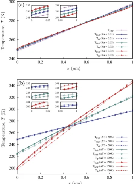
With elements in this size range, we need to see convergence of the hybrid method within 3 to 4 iterations for there to be any com-putational advantage over a full DSMC simulation. For this test case, we set the tolerance parameterftolto be 0.001.Fig. 3a shows
that, for all relaxation zone lengths, convergence of the method is reached within 4 iterations. However, convergence is not reached
within 4 iterations when the sampling zone lengths are 1kl or
3kl, as shown inFig. 3b. We therefore require larger sampling zones
of either 5klor 7kl, both of which provide convergence in only 2 to
3 iterations. Note that, for all simulations, the level of convergence fluctuates slightly due to noise. The converged temperature pro-files from the hybrid are shown inFig. 4; also plotted is the initial temperature fieldTNSF, and the full DSMC temperature fieldTFull.
The accuracy of the hybrid method is, however, more apparent from the mean percentage error at each iteration, presented in
Fig. 5. The error at iterationl= 0 is the error in the initial hydrody-namic NSF solution. It is seen that the final mean error is less than 0.1% when relaxation and sampling zone extents are both 5klor 7kl.
This accuracy is due to the hybrid method’s ability to capture the flux-correction field across the domain, as shown inFig. 6.
Essentially, the element size depends on the desired balance between accuracy and computational savings. Although sampling and relaxation zone extents of 7klprovide slightly higher accuracy,
we select an extent of 5klfor both zones. This provides a sufficient
level of accuracy while also enabling greater computational saving over a full-scale DSMC simulation. For the problems we study in this paper, each near-wall element therefore has a total extent of 10kl, while each bulk element has a total extent of 15kl.
3.2.2. Various rarefaction and temperature conditions
We now demonstrate the method’s ability to capture tempera-ture jump and the associated thermal Knudsen layer under various
rarefaction conditions (study A) and various temperature condi-tions (study B). In each test case, we maintain a wall separation
L¼1
l
m, and an average gas temperatureTav¼273 K.In study A, we consider the global Knudsen numbers:Kn= 0.01, 0.02, 0.03. This is achieved by varying the gas density for each case according to Eqs.(17) and (16). For all three cases, the temperature differenceDTbetween the walls is set to 50 K. In study B, we sim-ulate a range of temperature conditions by varying the tempera-ture difference between the walls:DT¼50 K, 100 K, 150 K. For all three cases, the gas density is set to maintainKn= 0.01. For every test case considered, bothKnand the temperature gradient are small enough that the bulk of the domain will be in equilib-rium. As in Section3.2.1, two near-wall elements should therefore be sufficient to capture the flux-correction field.
For all the cases, convergence of the hybrid solution occurs within 3 iterations to a tolerance parameter offtol¼0:001. This
is shown inFig. 7a and b, for studies A and B, respectively. In
Fig. 8a, we present the converged temperature profiles from all three hybrid simulations of study A, along with the corresponding full DSMC temperature profiles. Also shown is the initial NSF tem-perature profile: as this is independent ofKn, it is the same for all test cases in study A. Similarly, the converged temperature profiles from all three hybrid simulations of study B are shown inFig. 8b. The corresponding full-scale DSMC and initial NSF temperature profiles are also shown, with the NSF solution different for each value ofDT.
0 0.001 0.002 0.003 0.004
1 2 3 4
(a)
LRZ = 1λlLRZ = 3λl LRZ = 5λl LRZ = 7λl
0 0.001 0.002 0.003 0.004
1 2 3 4
(b)
LSZ = 1λl [image:9.595.44.273.67.205.2]LSZ = 3λl LSZ = 5λl LSZ = 7λl
Fig. 3.Convergence of the hybrid method for (a)LSZ¼5kland variousLRZ, and (b)
LRZ¼5kland variousLSZ.
255 270 285 300
0 0.2 0.4 0.6 0.8 1
(a)
TFull
TNSF
TΦ (LRZ = 1λl)
TΦ (LRZ = 3λl)
TΦ (LRZ = 5λl)
TΦ (LRZ = 7λl)
255 270 285 300
0 0.2 0.4 0.6 0.8 1
(b)
TFull
TNSF
TΦ (LSZ = 1λl)
TΦ (LSZ = 3λl)
TΦ (LSZ = 5λl)
TΦ (LSZ = 7λl) 248
249 250
0 0.01 0.02 296 297 298
0.98 0.99 1
248 249 250
0 0.01 0.02 296 297 298
0.98 0.99 1
Fig. 4.Final hybrid temperature solutionsTUfor (a)LSZ¼5kland variousLRZ, and (b)LRZ¼5kland variousLSZ. These are compared to the corresponding full DSMC temperature solutionTFull, and the hydrodynamic temperature solutionTNSF. Insets show results close to each wall.
0 0.1 0.2 0.3 0.4
0 1 2 3 4
(a)
LRZ = 1λlLRZ = 3λl LRZ = 5λl LRZ = 7λl
0 0.1 0.2 0.3 0.4
0 1 2 3 4
(b)
LSZ = 1λl [image:9.595.313.540.71.210.2]LSZ = 3λl LSZ = 5λl LSZ = 7λl
Fig. 5.Mean errorin the hybrid solutions for (a)LSZ¼5kland variousLRZ, and (b)
LRZ¼5kland variousLSZ.
0 0.2 0.4 0.6 0.8 1
0 0.2 0.4 0.6 0.8 1
(a)
Φx,FullΦx (LRZ = 1λl) Φx (LRZ = 3λl) Φx (LRZ = 5λl) Φx (LRZ = 7λl)
0 0.2 0.4 0.6 0.8 1
0 0.2 0.4 0.6 0.8 1
(b)
Φx,Full [image:9.595.39.279.252.452.2]Φx (LSZ = 1λl) Φx (LSZ = 3λl) Φx (LSZ = 5λl) Φx (LSZ = 7λl)
Fig. 6.Final hybrid flux-correction fieldsUxfor (a)LSZ¼5kland variousLRZ, and (b)
LRZ¼5kl and variousLSZ. These are compared with the full-scale DSMC flux-correctionUx;Full.
[image:9.595.313.540.262.431.2]Again, a clearer measure of accuracy is to consider the mean percentage error of the hybrid solution (compared with the corre-sponding full DSMC solution) at each iteration. This is presented in
Fig. 9and, for each case, the error at iterationl= 0 represents the error in the initial NSF solution. For all three values ofKnin study A, the hybrid technique reduces
to approximately 0.07% as shown in Fig. 9a. Fig. 10a shows that, for all Kn, the final hybrid flux-correction representation is in fairly good agreement with the cor-responding full DSMC flux-correction. However, asDTis increased in study B,Fig. 9b shows that the overall accuracy of the hybridmethod decreases. This is a reflection of the lower quality of the hybrid flux-correction representation, as seen inFig. 10b. However it should be noted that, for all values ofDT, the hybrid solution still provides a considerable improvement over the corresponding NSF solution.
For higher temperature gradients, the accuracy of the hybrid method could be improved by slightly increasing the extent of the near-wall elements (i.e. largerLRZandLSZ), or by adding an
ele-ment in the bulk. This would, however, reduce the computational savings obtained. As discussed in Section3.2.1, there must be a bal-ance exercised between the accuracy required from, and the com-putational speed-up offered by, the hybrid method.
3.2.3. Extreme temperature conditions
For the cases in Sections3.2.1 and 3.2.2, we used only two near-wall elements in our hybrid approach. However, even if the bulk of the domain is near-equilibrium, higher temperature conditions might result in a non-linear variation of conductivity with temper-ature. If so, the use of linear interpolation of the flux-correction field between opposite near-wall elements is not likely to produce the most accurate solution. Accuracy should be improved by the addition of micro elements within the bulk, i.e. increasing the micro resolution.
0 0.002 0.004 0.006
1 2 3 4
(a)
Kn = 0.01Kn = 0.02 Kn = 0.03
0 0.004 0.008 0.012
1 2 3 4
(b)
ΔT = 50K [image:10.595.55.283.66.230.2]ΔT = 100K ΔT = 150K
Fig. 7.Convergence of the hybrid method for (a) variousKn(study A), and (b) variousDT(study B).
240 260 280 300
0 0.2 0.4 0.6 0.8 1
(a)
TNSF TFull (Kn = 0.01) TΦ (Kn = 0.01) TFull (Kn = 0.02) TΦ (Kn = 0.02) TFull (Kn = 0.03) TΦ (Kn = 0.03)
200 220 240 260 280 300 320 340
0 0.2 0.4 0.6 0.8 1
(b)
TFull (ΔT = 50K) TNSF (ΔT = 50K) TΦ (ΔT = 50K) TFull (ΔT = 100K) TNSF (ΔT = 100K) TΦ (ΔT = 100K)
TFull (ΔT = 150K) TNSF (ΔT = 150K) TΦ (ΔT = 150K) 248
250 252
0 0.02 294 296 298
0.98 1
200 204
0 0.02 224
228 248 252
296 300
0.98 1 320 324 344 348
Fig. 8.Final hybrid temperature solutionsTUfor (a) variousKn(study A), and (b)
variousDT (study B). These are compared with the corresponding initial NSF temperature solutionsTNSF, and the corresponding full DSMC temperature solutions
TFull. Insets show results close to each wall.
0 0.5 1
0 1 2 3 4
(a)
Kn = 0.01Kn = 0.02 Kn = 0.03
0 0.5 1 1.5 2
0 1 2 3 4
(b)
ΔT = 50K [image:10.595.320.550.72.211.2]ΔT = 100K ΔT = 150K
Fig. 9.Mean errorin the hybrid solutions for (a) variousKn(study A), and (b) variousDT(study B).
-0.2 0 0.2 0.4 0.6 0.8 1 1.2
0 0.2 0.4 0.6 0.8 1
(a) Φx, Full (Kn = 0.01) Φx (Kn = 0.01) Φx, Full (Kn = 0.02) Φx (Kn = 0.02) Φx, Full (Kn = 0.03) Φx (Kn = 0.03)
-0.4 0 0.4 0.8 1.2 1.6 2 2.4
0 0.2 0.4 0.6 0.8 1
[image:10.595.323.551.259.455.2](b) Φx, Full (ΔT = 50K) Φx (ΔT = 50K) Φx, Full (ΔT = 100K) Φx (ΔT = 100K) Φx, Full (ΔT = 150K) Φx (ΔT = 150K)
Fig. 10.Final hybrid flux-correction fieldsUxfor (a) variousKn(study A), and (b) variousDT(study B), compared with the corresponding full DSMC flux-correction
Ux;Full.
[image:10.595.56.281.279.585.2]To verify the method’s ability to deal with more extreme tem-perature conditions, we consider a case where the global Knudsen
number is set to Kn= 0.01, but Tav is increased to 500 K. The
assumed value of
j
r is therefore increased to 0.027 W/m K(Younglove and Hanley, 1986). The temperature difference DT
between the walls is then set equal to 600 K (i.e. Tcold¼200 K
andThot¼800 K). We consider two hybrid configurations: in the
first, we have only two near-wall elements, i.e.P¼2; in the sec-ond, we add a bulk element in the centre of the system, i.e.P¼3. Settingftol¼0:01 for this test case, convergence occurs within 3
iterations for both configurations, as seen inFig. 11. The converged temperature profiles from both hybrid simulations, along with the initial NSF and the full-scale DSMC temperature profiles, are pre-sented inFig. 12.
[image:11.595.316.539.67.136.2]Once again, the accuracy of the hybrid is more clearly visible from the mean percentage error, shown for each iteration in
Fig. 13. As we would expect, the addition of a bulk micro element results in a more accurate temperature solution. In fact, in compar-ison with the initial NSF solution, this configuration provides an order of magnitude reduction in the mean error. This increased accuracy is the result of the higher quality flux-correction repre-sentation, as shown inFig. 14.
The accuracy of the hybrid could be further improved by increasing the molecular resolution either by increasing the ele-ment lengths, or by adding more bulk eleele-ments, or both. It should be noted however that even with only two near-wall elements the hybrid solution still provides a considerable improvement over the NSF solution.
3.2.4. Computational savings
In this paper we have not exploited time-scale separation — the full-scale and the hybrid element simulations are run for the same number of DSMC time-steps. Computational savings therefore come only from length-scale separation. The dimensions of the Fourier flow test cases considered here have been restricted by the need for a full-scale DSMC simulation in order to validate the hybrid method. With the degree of length-scale separation fairly small, the required micro elements occupy a significant portion of the domain. The computational savings provided by the hybrid on this particular heat transfer problem are therefore modest.
A measure of the computational speed-up Scan be obtained
from the ratio of the total processing time of the full DSMC approach, to the total processing time of the hybrid approach. For each simulation, the total processing time can be computed
from the total number of DSMC time-stepsM the average clock
time per DSMC time-steptc, i.e.
S¼ MFulltc;Full
MHybridtc;Hybrid
: ð19Þ
Note thatMis the total number of time-steps over both the tran-sient and steady-state periods and, for all cases in this paper,
MHybrid¼MFull¼53106. The computational cost of the hybrid
approach depends on both the micro resolution, and the number of iterations required. As the physical extent of each element is updated after each iteration based on the local mean free path, the average clock time per time steptcfor a particular element will
differ for each iteration. The total average clock time per time-step for the hybrid approachtc;Hybridis therefore calculated as the sum of
tcfor all micro elementsP, over all iterationsI, i.e.
tc;Hybrid¼
XI
l¼1
XP
k¼1 tcðk;lÞ
" #
: ð20Þ
For all test cases in Section3.2.2, our hybrid requires only two near-wall elements and convergence is reached inside 3 iterations. With
[image:11.595.47.269.389.452.2]P¼2 and I= 3, the computational speed-up S is presented in
Table 1 for each case. These speed-ups are determined by the extents of the near-wall elements,ðLSZþLRZÞleft andðLSZþLRZÞright
which are each 10kl. These extents during the final iteration (I= 3)
of each case are also presented in Table 1. If Kn= 0.01,
ðLSZþLRZÞleft and ðLSZþLRZÞright are small enough that we see a
0 0.02 0.04 0.06
1 2 3 4
Π = 2 Π = 3
Fig. 11.Convergence of the hybrid method forP¼2 andP¼3 elements.
200 300 400 500 600 700 800
0 0.2 0.4 0.6 0.8 1
TFull
TNSF
TΦ: Π = 2 TΦ: Π = 3
200 220
0 0.01 0.02 780 800
0.98 0.99 1
Fig. 12.Final hybrid temperature solutions TU, along with the initial NSF
temperature solutionTNSF, and the full DSMC temperature solutionTFull. Insets show results close to each wall.
0 2 4 6 8 10
0 1 2 3 4
[image:11.595.47.554.662.756.2]Π = 2 Π = 3
Fig. 13.Mean errorfor both hybrid configurations,P¼2 andP¼3.
-5 0 5 10 15 20 25
0 0.2 0.4 0.6 0.8 1 Φx, Full
Φx: Π = 2 Φx: Π = 3
[image:11.595.48.549.664.754.2]Fig. 14.Final hybrid flux-correction fieldsUx, and the full DSMC flux-correction fieldUx;Full.
Table 1
Computational speed-ups for the test cases of Section3.2.2.
Kngl DT(K) ðLSZþLRZÞleft(lm) ðLSZþLRZÞright(lm) I S
Study A
0.01 50 0.1 0.1 3 1.77
0.02 50 0.19 0.21 3 0.88
0.03 50 0.29 0.31 3 0.59
Study B
0.01 50 0.1 0.1 3 1.77
0.01 100 0.09 0.11 3 1.73
0.01 150 0.09 0.11 3 1.77
modest computational speed-up (S> 1). However, when Kn is increased to 0.02 and 0.03, these extents become larger so that we see no speed-up at all (S< 1).
Convergence of the multiscale method is also reached inside 3 iterations for both element configurations considered in Sec-tion3.2.3, whereKn= 0.01 andDT¼600 K. WithI= 3, the
compu-tational speed-ups for this case for both P¼2 and P¼3 are
shown inTable 2. For the configuration with only near-wall ele-ments,ðLSZþLRZÞleft andðLSZþLRZÞrightare again small enough for
us to see a modest computational speed-up. However, the increase in accuracy that comes with the addition of the bulk element increases the computational cost. In fact, with a bulk element lengthðLSZþ2LRZÞbulkcorresponding to 15kl, there is no
computa-tional speed-up at all, andS< 1.
In summary, while several cases in this paper demonstrate moderate computational savings from the hybrid method, a num-ber of cases are more computationally expensive than the equiva-lent full-scale DSMC simulation. It is important to note, however, that these Fourier flow cases have been chosen simply to test and validate the hybrid methodology itself. Future simulations of larger, more realistic, 2D and 3D problems will highlight any com-putational advantages of our multiscale approach. In transient flows, when temporal variations in the macroscopic property fields are much slower than the molecular time scales, computational savings can also be obtained by exploiting time scale separation, i.e. by controlling the time-steps in the macro and micro models as described byLockerby et al. (2013).
4. Conclusions
Based on a HMM–FWC approach, we have proposed a hybrid multiscale method that couples a continuum-fluid solver with the DSMC particle technique. The key advantage of this hybrid over existing continuum-DSMC hybrids is that DSMC micro elements of any size can be placed at any location in the flow, i.e. close to walls or in the bulk of the domain, independent of the continuum description. Therefore, unlike traditional HMM techniques, our method is able to simulate problems with any degree of scale sep-aration. The micro resolution can be adjusted for each problem to obtain the desired balance between accuracy and computational cost. Another useful feature of our approach is that the size of the micro elements adapts dynamically depending on the local mean free path of the gas.
For heat-transfer problems, the coupling in our method is per-formed through the computed heat fluxes. As a simple validation test, the method was demonstrated on micro Fourier flow. For a range of rarefaction and temperature conditions, we have shown the method’s ability to compensate for inaccurate boundary and constitutive information. The hybrid procedure was found to con-verge very quickly, inside 3 iterations for all test cases considered. Generally, good agreement with the equivalent full-scale DSMC simulations was observed, with the exact level of accuracy depend-ing on the micro element arrangement.
Due to the small degree of scale separation in the Fourier flow cases considered here, the computational speed-ups observed (over the full DSMC simulations) were modest. This problem was, however, selected only to provide a simple example on which
to test and validate the underlying methodology. Much greater speed-ups can be expected when simulating larger, more realistic engineering problems.
Before tackling 2D and 3D problems, the method needs to be developed to enable full coupling of mass and momentum, as well as heat transfer. Extension to 2D/3D then presents some additional challenges, including the application of mass, momentum, and heat transfer boundary conditions within 2D/3D relaxation zones, and 2D/3D interpolation of the correction fields between sampling zones. However, with this development, the method has the poten-tial to tackle a variety of problems, such as the flow of complex gas mixtures, or the flow through micro heat exchangers. The model-ling of thin bow shockwaves at the front of a planetary re-entry vehicle is another example which could benefit from the develop-ment of this hybrid as it encompasses both complex fluid behaviour (including chemical reactions of many gas species) and a high aspect ratio geometry. Our method also has the potential to be used in an inverse manner to obtain the transport properties of a gas.
Acknowledgements
This work is financially supported in the UK by EPSRC Pro-gramme Grant EP/I011927/1 and EPSRC Grants EP/K038664/1 and EP/K038621/1. Results were obtained using the ARCHIE-WeSt
High Performance Computer (www.archie-west.ac.uk) at the
Uni-versity of Strathclyde, funded by EPSRC Grant EP/K000586/1. SYD would like to thank Craig White and Alexander Patronis for their help and advice. The authors would also like to thank the reviewers of this paper for their very helpful comments.
References
Aktas, O., Aluru, N.R., 2002. A combined continuum/DSMC technique for multiscale analysis of microfluidic filters. J. Comput. Phys. 178 (2), 342–372.
Arlemark, E., Markelov, G., Nedea, S., 2012. Rebuilding of Rothe’s nozzle measurements with OpenFOAM software. J. Phys.: Conf. Ser. 362 (1), 012040. Asproulis, N., Kalweit, M., Drikakis, D., 2012. A hybrid molecular continuum method
using point wise coupling. Advan. Eng. Software 46 (1), 85–92.
Bird, G.A., 1998. Molecular Gas Dynamics and the Direct Simulation of Gas Flows. Oxford Engineering Science Series. Clarendon Press.
Borg, M.K., Macpherson, G.B., Reese, J.M., 2010. Controllers for imposing continuum-to-molecular boundary conditions in arbitrary fluid flow geometries. Mol. Simulat. 36 (10), 745–757.
Borg, M.K., Lockerby, D.A., Reese, J.M., 2013. A multiscale method for micro/nano flows of high aspect ratio. J. Comput. Phys. 233, 400–413.
Borg, M.K., Lockerby, D.A., Reese, J.M., 2013. Fluid simulations with atomistic resolution: a hybrid multiscale method with field-wise coupling. J. Comput. Phys. 255, 149–165.
Delgado-Buscalioni, R., Coveney, P.V., 2003. Continuum–particle hybrid coupling for mass, momentum, and energy transfers in unsteady fluid flow. Phys. Rev. E 67, 046704.
Flekkøy, E.G., Wagner, G., Feder, J., 2000. Hybrid model for combined particle and continuum dynamics. Europhys. Lett. 52 (3), 271.
Garcia, A.L., Bell, J.B., Crutchfield, W.Y., Alder, B.J., 1999. Adaptive mesh and algorithm refinement using direct simulation Monte Carlo. J. Comput. Phys. 154 (1), 134–155.
Hadjiconstantinou, N.G., Patera, A.T., 1997. Heterogeneous atomistic-continuum representations for dense fluid systems. Int. J. Modern Phys. C 8 (4), 967–976. Hash, D.B., Hassan, H.A., 1996. Assessment of schemes for coupling Monte Carlo and Navier–Stokes solution methods. J. Thermophys. Heat Transfer 10 (2), 242–249. Kessler, D.A., Oran, E.S., Kaplan, C.R., 2010. Towards the development of a multiscale, multiphysics method for the simulation of rarefied gas flows. J. Fluid Mech. 661, 262–293.
Lian, Y.-Y., Tseng, K.-C., Chen, Y.-S., Wu, M.-Z., Wu, J.-S., Cheng, G., 2008. An improved parallelized hybrid DSMC–NS algorithm. In: Proceedings of the 26th International Symposium on Rarefied Gas Dynamics, Kyoto, Japan, vol. 1084 (1), pp. 341–346.
Lockerby, D.A., Duque-Daza, C.A., Borg, M.K., Reese, J.M., 2013. Time-step coupling for hybrid simulations of multiscale flows. J. Comput. Phys. 237, 344–365. Lofthouse, A.J., 2008. Nonequilibrium Hypersonic Aerothermodynamics using the
Direct Simulation Monte Carlo and Navier–Stokes Models. Ph.D. thesis, University of Michigan.
[image:12.595.42.294.87.133.2]O’Connell, S.T., Thompson, P.A., 1995. Molecular dynamics – continuum hybrid computations: a tool for studying complex fluid flows. Phys. Rev. E 52, R5792– R5795.
Table 2
Computational speed-ups for the configurations of Section3.2.3.
P ðLSZþLRZÞleft
(lm)
ðLSZþ2LRZÞbulk
(lm)
ðLSZþLRZÞright
(lm)
I S
2 0.07 – 0.12 3 1.71
3 0.07 0.15 0.12 3 0.96
OpenFOAM Foundation, 2013.www.openfoam.org. URL<www.openfoam.org>. Patronis, A., Lockerby, D.A., Borg, M.K., Reese, J.M., 2013. Hybrid continuum–
molecular modelling of multiscale internal gas flows. J. Comput. Phys. 255, 558– 571.
Ren, W., E, W., 2005. Heterogeneous multiscale method for the modeling of complex fluids and micro-fluidics. J. Comput. Phys. 204 (1), 1–26.
Roveda, R., Goldstein, D.B., Varghese, P.L., 1998. Hybrid Euler/particle approach for continuum/rarefied flows. J. Spacecraft Rockets 35, 258–265.
Scanlon, T.J., Roohi, E., White, C., Darbandi, M., Reese, J.M., 2010. An open source, parallel DSMC code for rarefied gas flows in arbitrary geometries. Comput. Fluids 39 (10), 2078–2089.
Schwartzentruber, T., Scalabrin, L., Boyd, I., 2007. A modular particle–continuum numerical method for hypersonic non-equilibrium gas flows. J. Comput. Phys. 225 (1), 1159–1174.
Sun, Q., Boyd, I.D., 2002. A direct simulation method for subsonic, microscale gas flows. J. Comput. Phys. 179 (2), 400–425.
Sun, Q., Boyd, I.D., Candler, G.V., 2004. A hybrid continuum/particle approach for modeling subsonic, rarefied gas flows. J. Comput. Phys. 194 (1), 256–277. von Smoluchowski, M., 1898. Ueber wärmeleitung in verdünnten gasen. Ann. Phys.
300 (1), 101–130.
Wadsworth, D.C., Erwin, D.A., 1990. One-dimensional hybrid continuum/particle simulation approach for rarefied hypersonic flows. In: Proceedings of the 5th AIAA/ASME Joint Thermophysics and Heat Transfer Conference, Seattle, WA. Werder, T., Walther, J.H., Koumoutsakos, P., 2005. Hybrid atomistic-continuum
method for the simulation of dense fluid flows. J. Comput. Phys. 205 (1), 373– 390.
White, C., Borg, M.K., Scanlon, T.J., Reese, J.M., 2013. A DSMC investigation of gas flows in micro-channels with bends. Comput. Fluids 71, 261–271.
Wijesinghe, H.S., Hornung, R.D., Garcia, A.L., Hadjiconstantinou, N.G., 2004. Three-dimensional hybrid continuum-atomistic simulations for multiscale hydrodynamics. J. Fluids Eng. 126 (5), 768–777.
Wu, J.-S., Lian, Y.-Y., Cheng, G., Koomullil, R.P., Tseng, K.C., 2006. Development and verification of a coupled DSMC–NS scheme using unstructured mesh. J. Comput. Phys. 219 (2), 579–607.
Yasuda, S., Yamamoto, R., 2008. A model for hybrid simulations of molecular dynamics and computational fluid dynamics. Phys. Fluids 20 (11), 113101. Younglove, B.A., Hanley, H.J.M., 1986. The viscosity and thermal conductivity
coefficients of gaseous and liquid argon. J. Phys. Chem. Ref. Data 15, 1323–1337.