Network fault analysis with increased distributed generation penetration and evaluation of solutions to issues caused by distributed generation

(1)

warwick.ac.uk/lib-publications

A Thesis Submitted for the Degree of PhD at the University of Warwick Permanent WRAP URL:

http://wrap.warwick.ac.uk/99672

Copyright and reuse:

This thesis is made available online and is protected by original copyright. Please scroll down to view the document itself.

Please refer to the repository record for this item for information to help you to cite it. Our policy information is available from the repository home page.

(2)

Network Fault Analysis with Increased

Distributed Generation Penetration and

Evaluation of Solutions to Issues

Caused by Distributed Generation

By

Han Qin

A Thesis Submitted for the Degree of

Doctor of Philosophy

School of Engineering

The University of Warwick

(3)

i

List of Figures

Figure 1. 1 Power system structure……….…3

Figure 1. 2 Diagram of a typical distribution network in radial (open ring) structure…...…4

Figure 2. 1 Voltage variation down a radial feeder……….………...13

Figure 2. 2 Simple two-bus radial distribution network………...….14

Figure 2. 3 Configuration of a gas turbine CHP ………..……..19

Figure 2. 4 Configuration of fuel cell CHP ………..…...20

Figure 2. 5 Fixed speed induction generator wind turbine ………..…..24

Figure 2. 6 Figure 2.6 DIFIG wind turbine ………...24

Figure 2. 7 Figure 2.7 Full power converter wind turbine ……….……25

Figure 2. 8 Figure 2.8 Grid-connected small PV inverter ………..………...26

Figure 2. 9 Diagram of a fault-ride through………..…...31

Figure 2. 10 Topology of a two-level VSC………..………..35

Figure 2. 11 Installation locations of shunt compensator in a power system………..……...36

Figure 2. 12 Diagram of SVC in a power system………..……...37

Figure 2. 13 Site View, Barnstable SVC ………..38

Figure 2. 14 Diagram of a STATCOM………..40

Figure 2. 15 ABB PCS 6000 6-16MVA STACTOM ………...40

Figure 2. 16 Installation locations of series compensator in a power system……….41

Figure 2. 17 (a) GTSC, (b) TCSC and (c) TSSC………42

Figure 2. 18 Diagram of a SSSC………...43

Figure 2. 19 Diagram of a B2B VSC……….45

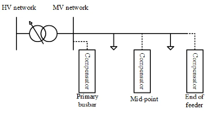
Figure 2. 20 FCL installation at the primary busbar………..46

Figure 2. 21 FCL installation at the feeder………47

Figure 2. 22 FCL installation at the interconnection between two primary busbars………..47

Figure 2. 23 Drawing and complete 3-phase- FLC 12-800 system after installation in Boxberg, Germany ………...49

Figure 2. 24 Fault current limiting by a RSFCL ………49

Figure 2. 25 Diagram of a three-phase FCL ………50

Figure 2. 26 Fault current limiting of a saturated iron-core FCL ………...51

Figure 3. 1 Common types of fault………53

Figure 3. 2 Short circuit current far-from-generator with constant ac component………….55

Figure 3. 3 Example of fault in a radial network………56

Figure 3. 4 Fault fed from a single source and the equivalent circuit ………..59

Figure 3. 5 Split-phase winding induction motor………..65

Figure 3. 6 Capacitor-start induction motor………..66

Figure 3. 7 Per phase equivalent circuit of induction motor………..67

Figure 3. 8 Torque associated with two revolving fields and output torque of single-phase induction machine ………67

Figure 3. 9 Circuit diagram of the short circuit test equipment………..74

(7)

v

Figure 3. 11 Indicative simulation model………..77

Figure 3. 12 Impact of transformer impedance on (a) make and (b) break fault current contributions by loads………...80

Figure 3. 13 Normalised fault current contribution of load………...82

Figure 3. 14 Circuit diagram for simulation………..84

Figure 3. 15 Estimated maximum make fault current compositions………90

Figure 3. 16 Estimated minimum make fault current compositions………..90

Figure 3. 17 Estimated maximum break fault current compositions………91

Figure 3. 18 Estimated maximum break fault current compositions………91

Figure 3. 19 Estimated band of make fault current compositions………..92

Figure 3. 20 Estimated band of break fault current compositions………..92

Figure 3. 21 Initial symmetrical fault current contribution to 400V network of different size synchronous machines………..98

Figure 3. 22 Initial symmetrical fault current contribution to 11kV network of different size synchronous machines………..99

Figure 3. 23 Model of radial distribution network………...101

Figure 3. 24 (a) Voltage variation and (b) fault level caused by DG at different locations in an 11kV network……….103

Figure 3. 25 Short circuit current close to power plant………104

Figure 3. 26 dc and ac components of the short circuit current from a synchronous machine ………106

Figure 3. 27 ac components of synchronous machine short circuit current……….107

Figure 3. 28 Ratio of sub-transient current to total current of synchronous machine ………108

Figure 3. 29 Zero-crossing time of short circuit current for different time constant ratios………...110

Figure 3. 30 Time constant ratios for synchronous generators in different sizes………….111

Figure 4. 1 Single line diagram of the simplified model………..119

Figure 4. 2 Fault level composition of Group 1………...121

Figure 4. 6 Normalized fault level change of Group 1……….124

Figure 4. 10 Fault level composition when DG penetration level is increasing of Group 1 ………130

(8)

vi

Figure 4. 14 Predicted power demand changes - Gone Green……….133

Figure 4. 15 Predicted power demand changes - No Progression………134

Figure 4. 16 Domestic lighting technology estimation - Gone Green………..137

Figure 4. 17 Domestic lighting technology estimation - No Progression………137

Figure 4. 18 Average lighting power demand of a single house in the UK………..139

Figure 4. 19 Average power demand of different types of domestic appliance - Gone Green ………140

Figure 4. 20 Average power demand of different types of domestic appliance - No Progression ………141

Figure 4. 21 Average power difference between two scenarios………...141

Figure 4. 22 Working cycle of heat-pump………...143

Figure 4. 23 Estimated UK resident house growth………..144

Figure 4. 24 Estimation of numbers of different types of electrical powered heaters - Gone Green ……….………145

Figure 4. 25 Estimation of numbers of different types of electrical powered heaters - No Progression ………145

Figure 4. 26 Average Electrical Power Demand in House Heating………146

Figure 4. 27 Estimated load composition - Gone Green……….148

Figure 4. 28 Estimated load composition - No Progression………148

Figure 4. 29 Estimated number of electrical vehicle on road ………..150

Figure 4. 30 Percentage of electrical vehicle in total load demand ………151

Figure 4. 31 Indication of electrical vehicle charger circuit………151

Figure 4. 32 Estimated fault level contribution - Gone Green………155

Figure 4. 33 Estimated fault level contribution - No Progression………155

Figure 4. 34 Estimated load composition - Gone Green……….156

Figure 4. 35 Estimated load composition - No Progression……….156

Figure 4. 36 General Load Fault Level Contribution (MVA/MVA) – Gone Green………157

Figure 4. 37 General Load Fault Level Contribution (MVA/MVA) - No Progression ………157

Figure 4. 38 Estimated general load fault level contribution – Gone Green………..158

Figure 4. 39 Estimated general load fault level contribution – No Progression…………..158

Figure 5. 1 Topology 1 using shunt thyristor crowbar in SSSC protection……….167

Figure 5. 2 Topology 2 using shunt thyristor crowbar in SSSC protection………168

Figure 5. 3 SLD for the 11kV distribution network……….170

Figure 5. 4 Total fault current of Topologies 1 and 2………..171

Figure 5. 5 Fault detection using voltage reference………174

Figure 5. 66 Fault detection using current reference………175

Figure 5. 7 Results for fault detection speeds using voltage and current reference………175

Figure 5. 8 Equivalent circuit of a transformer referring to the primary winding…………177

Figure 5. 9 Core magnetic flux density during fault………179

Figure 5. 10 Voltage of the SSSC during fault……….181

Figure 5. 11 Magnetic flux density of the transformer with doubled primary winding leakage inductance and 3.5 km cable length………181

(9)

vii

Figure 5. 13 Voltage of the SSSC during fault (protection failure)………183

Figure 5. 14 Calculated magnetic flux density of the transform core during fault (protection failure) ………...183

Figure 5. 15 Foster thermal equivalent circuit model………186

Figure 5. 16 Cauer thermal equivalent circuit model……….186

Figure 5. 17 Structure of the surge current test model………192

Figure 5. 18 Cauer model for thyristor with heat sink………193

Figure 5. 19 Test circuit………..194

Figure 5. 20 Thyristor crowbar surge current test bench……….194

Figure 5. 21 Case temperature during experiment @ 300A RMS………..195

Figure 5. 22 Case temperature simulation vs experiment (Heat sink 2)……….196

Figure 5. 23 Forward voltage during turning on simulation vs experiment………196

Figure 5. 24 Junction temperature in the surge current test……….200

Figure 5. 25 Case temperature in the surge current test………..200

Figure 5. 26 Fault passing through the thyristor crowbar of the SSSC with transformer - Topology 1………..204

Figure 5. 27 Fault current passing through the thyristor crowbar of the transformerless SSSC - Topology 1………204

Figure 5. 28 Tj of forward thyristor (1km cable and 25°C) - Topology 1……….205

Figure 5. 29 Tj of reverse thyristor (1km cable and 25°C) - Topology 1……….205

Figure 5. 32 Tj of forward thyristor (10km cable and 25°C) - Topology 1………207

Figure 5. 33 Tj of reverse thyristor (10km cable and 25°C) - Topology 1………207

Figure 5. 35 Tj of reverse thyristor (10km cable and 40°C) - Topology 1………208

Figure 5. 36 Tj of forward thyristor (1km cable and 25°C) - transformerless SSSC, Topology 1………..210

Figure 5. 37 Tj of reverse thyristor (1km cable and 25°C) - transformerless SSSC, Topology 1………..210

(10)

viii

Figure 5. 45 Fault passing through the thyristor crowbar of transformerless SSSC - Topology

2………..215

Figure 5. 46 Tj of forward thyristor (1km cable and 25°C) - Topology 2………..….216

Figure 5. 47 Tj of reverse thyristor (1km cable and 25°C) - Topology 2………..….216

Figure 5. 48 Tj of forward thyristor (1km cable and 40°C) - Topology 2………..….217

Figure 5. 49 Tj of reverse thyristor (1km cable and 40°C) - Topology 2………..….217

Figure 5. 55 Tj of reverse thyristor (1km cable @ 25°C)-transformerless SSSC, Topology 2………..220

Figure 5. 56 Tj of forward thyristor (1km cable @ 40°C)-transformerless SSSC, Topology 2………..221

Figure 6. 1 The 11kV distribution network model……….226

Figure 6. 2 Schematic diagram of the control system of the right-hand side VSC of the B2B……….228

Figure 6. 3 Plane graph of dq0 coordinates system………229

Figure 6. 4 Block diagram of the phase-locked loop………...232

Figure 6. 5 Block diagram of the dc voltage control loop………235

Figure 6. 6 Block diagram of the current control loop……….238

Figure 6. 7 Voltage of load busbar 13 at minimum load with increasing DG penetration………..239

Figure 6. 8 Voltage variation at load busbar 13 with interconnection using a B2B-VSC power electronic controller to transfer power………240

Figure 6. 9 Fault current limiting using B2B-VSC for the interconnection………241

Figure 6. 10 Single line diagram of a network with imbalanced feeder loadings………….245

Figure 6. 11 Total network loss reductions under different DG penetrations……….246

Figure 7. 1 Eddy current………..252

Figure 7. 2 Schematic of the hysteresis curve………254

Figure 7. 3 Schematic of the transformer core with winding current I………..255

(11)

ix

Figure 7. 5 Schematic of a saturated iron core FCL……….257

Figure 7. 6 Schematic of B-H curve………259

Figure 7. 7 Test circuit of open circuit test of the transformer core………262

Figure 7. 8 Test circuit of the loss test……….262

Figure 7. 9 Test bench ………263

Figure 7. 10 Transformer core hysteresis loop………264

Figure 7. 11 Hysteresis loop - normal status………266

(12)

x

List of Tables

Table 2. 1 Limits for harmonic emission ………..28

Table 2. 2 Settings for long-term parallel operation ………29

Table 2. 3 Settings for infrequent short-term parallel operation ………..29

Table 2. 4 Short circuit parameters ………..32

Table 3. 1 Voltage factor c ………..58

Table 3. 2 Parameters of four single-phase induction motors………73

Table 3. 3 Results of the short circuit current calculation for four single-phase induction motors………...73

Table 3. 4 Typical compositions of domestic, commercial and industrial loads………78

Table 3. 5 Parameters of transformer and induction machines in the model………..78

Table 3. 6 Reference fault current contribution……….81

Table 3. 7 Fitting coefficients for different types of loads……….83

Table 3. 8 Cable parameters………..83

Table 3. 9 Short circuit current with distribution cable………..85

Table 3. 10 Typical composition of general load………...86

Table 3. 11 Sample substation data………...………89

Table 3. 12 Substation specified fault current contribution………..89

Table 3. 13 Mean normalized break FL contributions of synchronous generators to 400V and 11kV networks (MVA/MVA)………97

Table 3. 14 Zero-crossing time of fault current in 11kV network with fault at DG site ………112

Table 3. 15 Zero-crossing time of fault current with different distance between fault and DG ………113

Table 3. 16 Zero-crossing time of fault current contributed by different numbers of generators ………114

Table 4. 1 Average annual power consumption and rated power of different types of lighting ………136

Table 4. 2 Appliances of different types of appliance ………140

Table 4. 3 Normalized fault level contribution of commercial and industrial loads (MVA/MVA) ………153

Table 5. 1 Functions of commonly used power electronic compensators in SOP ………163

Table 5. 2 Construction cost comparison between B2B VSC and STATCOM/SSSC ………..164

Table 5. 3 Comparison between B2B VSC and STATCOM/SSSC ………..165

Table 5. 4 Parameters for 11kV network model……….170

Table 5. 5 Transformer parameters……….179

Table 5. 6 Experiment equipment parameters……….195

Table 5. 7 Ratings of different types of thyristors………198

Table 5. 8 Foster thermal resistance of different type of thyristors………199

(13)

xi

Table 5. 10 Case details………...202

Table 5. 11 Thyristor models ………202

Table 6. 1 Network loss reduction (kW) at DG penetration of 20%...246

Table 7. 1 Permeability of common materials ………260

Table 7. 2 Transformer core parameter………...261

Table 7. 3 Loss test measurements……….264

Table 7. 4 Fitting coefficients ………265

(14)

xii

Declaration

This thesis submitted to the University of Warwick in support of the application for the degree of Doctor of Philosophy. Not any parts or in whole has been send to other degree or qualifications at any other university. The work presented in Chapter 3 and Chapter 4 has been written in the deliverables and reported to the Project of FlexDGrid, WPD. Parts of the work in Chapter 3 and Chapter 6 are published by the author in peer reviewed research papers listed. The work described in this thesis is carried out by the author in the School of Engineering of the University of Warwick, unless is commonly understood or referenced in the text.

Han Qin

(15)

xiii

Acknowledgement

I would like to give my sincerely thank to all people and organisations who offered help and supports to me during my PhD study. Among them, there are some persons I would like to present my thankfulness individually.

First and foremost, I would like to present my most gratefully and sincerely thanks to my supervisor, Professor Li Ran, for all his help, encouragement, guidance and care during my whole PhD study in the University of Warwick. During this time, he played lots of important roles to me. Firstly, he is a wise and patient supervisor in my academic experience. From the very beginning when I applied the PhD study to the final stage of my thesis writing, Li has always been patient and kind to offer his professional supervision to my work. He is also very strict to my works with high standard. Though I know it is still a long way for me to reach his requirement, I have seen my improvements thanks to Li’s effort. Secondly, he is like a guide in my life. He shares his life experience with me and lead me to the right direction when I feel confused in my life. Finally, he is also a kind elder for all his students. He always cares about all his students’ personal life and treats us like his own children. I would like to thank Li for helping me to overcome the difficulties and challenges in the study.

Secondly, I would like to thank the School of Engineering, University of Warwick to offer me the opportunity to have my PhD study here with all the software and hardware supports in my study. I would also like to send my appreciation to the Western Power Distribution (WPD) for offering me the opportunity to attend the FlexDGrid project and the scholarship for my PhD study.

Also, I would like to thank my second supervisor Dr. Olayiwola Alatise for his help in the FleDGrid project. I would like to thank my colleagues, Dr. Mohamed Abdel Motalab Ali Soli Ahmad and Dr. Qian Zhou for their supports and help in the FlexDGrid project and I really enjoyed working with them. Here I would like to deeply mourn Qian who has passed away due to cancer in 2016.

(16)

xiv

Finally, and most importantly, I would like to thank my beloved family and devote this work to them. I would like to send my grateful and sincerely thanks to my mother Xiangdong Han and my father Chaoyun Qin for all the supports, understanding and love to me during my whole study period abroad. They devote all their love to me without anything in return. I am proud to have them and will try to be the proud of them. I wish them to know that I do and will always love them. I would also like to thank my grandparents, uncles, aunts and cousins. Thank them for loving me. Last but not the least, I would like to give my thank to my lovely and beautiful friend, Manyuan Li. Thanks for accompanying and supporting me during the time, and all the happiness and tears we had together.

Han Qin

(17)

xv

Abstract

(18)

xvi

Nomenclature

ac alternative current

ANSI American National Standards Institute ASHP air source heat pump

B2B VSC back to back voltage source converter BJT bipolar juction transistor

CFL comact fluorescent light CHP combined heat and power

CIGRE Conference on Large High Voltage Electric System CIRED Conference on Electricity Distribution Networks dc direct current

DFIG double fed induction generator DG distributed generation

DNO distribution network operator ER G74 Engineering Recommendation G74

ESQCR Electricity Safety, Quality and Continuity Regulations EU Europe Union

EV electrical vehicle

FCC fault current contribution FCL fault current limiter FES Future Energy Scenarios FL fault level

FLC fault level contribution GDHP ground source heat pump GTO gate turn-off thyristor

HTSFCL high temperature superconducting fault current limiter HV high voltage

HVAC high voltage alternative current HVDC high voltage direct current

IEC International Electrotecnical Commission IGBT insulated gate bipolar thyristor

IGCT integrated gate communicated thyristor LED light-emitting diode

LV low voltage

MPPT maximum power point tracking MV medium voltage

n hatmonic order NGC National Grid Code NGS National Grid System O/f over frequency O/V over voltage pf power factor

PI proportional and integral feedback PL penetration level

PV photovoltaic

(19)

xvii RMS root mean square

SP Scottish Power

SPWM sinusoidal pulse width modulation SSSC static series sychronous compensator STATCOM static synchronous compensator SVC static Var compensator

TOUT Time of Use Tariffs U/f under frequency U/V under voltage

VSC vlotage source converter

[xabc] matrix expression of quantities in abc coordinates [xdq] matrix expression of quantities in dq0 coordinates ∆I difference between results from different methods ∆V21 voltage rise at load busbar in per unit system As swept area of rotor disk

As initial value of aperiodic C capacitance of a capacitor c voltage factor

Cp power efficient D stator bore diametre E energy stored in a capacitor Ed.c. energy stored in the d.c. bus eoff turn off loss

eon turn on loss

erec diode reverse recovery energy Etotal total energy loss

f frequency

F(s) square of the d.c. bus voltage FCCref referemce fault current contribution

FLbreak break fault level contribution of sychronous machine FLC normalised fault level contribution

FLC'break normalised fault level cotrinution of sychronous machine through transformer FLCbreak normalised break fault level contribution of sychronous machine

Fref(s) reference voltage input for the d.c. bus voltage control loop g acceleration due to gravity

Gd.c.(s) gains of the PI controller for the d.c. bus voltage control loop GPLL(s) gains of the PI controller for the phase-locked loop H effective head

I phase current at rated output power Ib symmetrical current

Ibreak break fault current ic collector current id d-axis current

Idc dc component of short circuit current If fault current

if diode foreard current

(20)

xviii Ifi fault current component

IfM fault current contributed by rotating load Ifup fault current contributed by upstream network Ik'' initial symmetrical short circuit current Im magnetising current

Imake make fault current Ip peak short circuit current

Ip' simulated value of peak short circuit current Ip'' measured value of peak short circuit current iq q-axis current

Ir rated current of small scale induction machine

Isc_break break short circuit current of synchronous machine Isc_subtransient subtransient short circuit of sychronous machine K1 adjacent coeffiecient

K2 adjacent coeffiecient

KId.c. integation gain factor for the d.c. bus voltage control loop KIG integation gain factor for the phase-locked loop

KPd.c. propotional gain factor for the d.c. bus voltage control loop KPG propotional gain factor for the phase-locked loop

L stator length

Lf inductance of the filter P power output

P real power flowing into the d.c. bus P(s) power flowing into the d.c. bus p.u. per unit system

PDG real power output of DG pf load power factor

PL2 real power comsumed by load Pn rated power capacity

Q flow rate

Q reactive power flowing into the d.c. bus QDG reactive power input/output of DG QL2 reactive power consumed by load R cable resistence

R' transient resistance

R1 resistance of the primary winding R2 resistance of the secondary winding Rc core loss resistance

Rf resistance of the filter

Rf Thevenin equivalent resistance of the fault

RL Thevenin equivalent resistance of the transmission line Rm magnitizing resistance

Rr' induction machine per phase rotor winding resistance with respect to the stator winding Rs Thevenin equivalent resistance of the source

Rs induction machine per phase stator winding resistance RT Thevenin equivalent resistance of the transformer s rotor slip

(21)

xix Sr rated capacity of sychronous machine

t time

T(θ) transformation matrix of θ tf turn off time

tr turn on time

trr reverse recovery time ud d-axis voltage

Un norminal phase to phase voltage at fault location uq q-axis voltage

Ur rated voltage of sychronous machine v wind velocity

V voltage over the capacitor V1 primary busbar voltage V2 load busbar voltage vabc grid voltage vce on-state voltage vd.c. d.c. bus voltage vfabc voltage of the filter vfabc diode formward voltage vgd d-axis voltage of vabc vgq q-axis voltage of vabc VL norminal line voltage

Vm peak amplitude of the norminal voltage of the grid Vn norminal voltage

vq q-axis component Vφ-n phase to netural voltage Vφ-φ phase to phase voltage X cable reactance X' transient reactance X/R reactance/resistance ratio

X1 reactance of the primary winding X2 reactance of the secondary winding

Xd'' d-axis subtrainsient reactance of sychronous machine

xd'' per-unit d-axis subtransient reactance of sychronous machine xe error of the reference and feedback

Xf Thevenin equivalent reactance of the fault Xkl'' initial positive sequence reactance

XL Thevenin equivalent reactance of the transmission line xL per-unit leakage reactance of the windings

XL leakage reactance

xL per-unit leakage reactance Xm magnetiszing reactance Xm magnetising reactance

xmd per-unit d-axis magnetising reactance

Xr' induction machine per phase rotor winding reactance with respect to the stator winding Xs Thevenin equivalent reactance of the source

(22)

xx Z' transient impedance

ZDG Thevenin equivalent impedance of DG Zf Thevenin equivalent impedance of the fault Zload Thevenin equivalent impedance of load Zs Thevenin equivalent impedance of source Zt equivalent transformer impedance

δ ration of a load to the total load η overall efficiency

θ time dependent angle between d-axis and α-axis θ0 angular velocity of Park Trasformation

θref(s) reference angular velocity inputed for the phase-locked loop κ calculation factor

ξ damping factor for the phase-locked loop

ξd.c. damping factor for the d.c. bus voltage control loop ρ density of certain material

τa.c. a.c. time constant of ac component in short-circuit current by sychronous machine φ0 assummed initial angle between d-axis and α-axis

(23)

1

Introduction

1

1.1 History of Electrical Power System

The world’s first power station was built at Cragside, England, designed by Lord Armstrong

in 1868. It supplied power to the daily usage for private farm buildings using water powered

Siemens dynamos. In January 1882, the first public power station, Holborn Viaduct

Generating Station, started to operate at London. It was a project of Thomas Edison and the

station supplied power at 100 V driven by a steam engine [1]. The first central generating

station was later built in Pearl Street in New York, also by Thomas Edison in 1882. It

supplied power at 110V using a steam powered generator [2]. All these three stations

(24)

2

The first full alternating current (ac) power system in the world was built by William

Stanley in Great Barrington, Massachusetts in 1886 [3]. The first ac station in Great Britain

was opened at Deptford and transmitted at 10kV to customers in London in 1891 [4]. In the

same year, the first three-phase ac transmission system from Lauffen to Frankfurt was built

in Germany by Oskar von Miller. The transmission system was at 40Hz and 15kV, covering

a distance of 109 miles (175km) [5]. Thereafter, centralized generation and three-phase ac

power system have gradually developed into the structure today and been used for electrical

power supply in the world.

In the recent decades, the high voltage dc (HVDC) technology has been studied and

developed by many researchers and engineers. This was driven by [6]:

1) The need to transmit large amount of electricity over a very long distance due to the

energy resources far from the load centres;

2) More cost-effective of long distance HVDC compared to HVAC transmission; and

3) The increasing amount of offshore wind power generation is to be transmitted back

to the in-land load centres.

The development of HVDC accelerates the utilisation of power electronic devices in

the power system. Additionally, the number of distributed generation (DG) is increasing with

(25)

3

1.2 Brief Introduction to Distribution Network

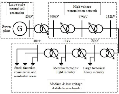
An electric power system consists of three major components: generation system (large

central power plants), transmission system and distribution system. Each component has its

typical voltage level and is connected to another component through step up/down power

[image:25.595.141.554.388.715.2]

transformers, the structure is indicated in Figure 1.1.

(26)

4

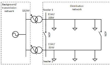
Typically, a distribution network (400V to 33kV phase to phase nominal voltage) starts

from the distribution substation fed by several transmission lines from the transmission

system [7]. The typical primary distribution substation at the bulk supply point uses two to

four 50MVA 132/11kV step-down transformers, depending on the supplied peak load, to

supply an area of 3-6 square miles in the UK [8]. The topology of a distribution network is

[image:26.595.140.576.355.613.2]

typically designed in radial (open ring) structure, as indicated in Figure 1.2.

(27)

5

Circuit breakers are used to connect branches that when the circuit breaker closes, the

radial structure can be transformed into a loop structure to improve the reliability in

delivering power to the customers. Fuses and circuit breakers are connected in series in the

network to provide protection against the occurrence of short circuits (faults). The ratings of

the protection equipment are originally designed to withstand short circuit current from both

upstream and downstream dynamic loads without DG in the past. However, with the

increasing energy demand and global climate change, the distribution network nowadays is

adopting more DGs installed by the electrical energy customers. These changes have brought

about a number of issues in network operation and management for the distribution network

operators (DNOs).

1.3 Brief Introduction to Distributed Generation

The arrangement using centralised generation and high voltage transmission has been

adopted in the modern electrical power system development over the past 90 years [9]. This

arrangement has a number of advantages. The centralised large generating units can be made

efficient in the electricity generation with relatively small number of staff in the operation.

The high voltage transmission network allows the generating plants to be dispatched at any

time and limits the electrical losses over long distance transmission. The distribution network

can be designed simply for unidirectional power flow and sized to accommodate customer

(28)

6

Since the early 1990s, a revival of interests in connecting generation to the distribution

network has been raised in response to the increasing load demand and global warming. This

type of generation has been named, from different aspects, as [11]:

• Dispersed generation to distinguish it from centralised generation;

• Distributed generation since the generation units are connected in the distribution

network; or

• Embedded generation from the concept of generation embedded in the distribution

network.

These three terms can be considered synonymous and interchangeable. The use of these

terms is mainly regional.

Investigations on DG have been conducted by working groups of both the International

Conference on Large High Voltage Electric System (CIGRE) on 1997 and the International

Conference on Electricity Distribution Networks (CIRED) on 1998 and 1999 [12-14]. The

reports of both working groups pointed out that there is no universally accepted definition

of DG but some common attributes may be listed as:

• Not centrally planned or despatched,

• Sizing between 50kW to 100MW, and

• Connected to the distribution network.

The review of technologies of DG and the impacts of DG on the network is made in the

(29)

7

1.4 Research Objectives and Contributions

Due to increasing DG penetration, voltage and fault level issues are caused by DG in the

distribution network. Aiming at eliminating these issues, more accurate estimations of the

network fault level, at present and in the future, are required. Furthermore, solutions are

proposed by employing fault current limiter (FCL) and soft open point (SOP) into the

distribution network. Evaluations to these solutions are also required regarding the operation

loss. Regarding the former issues, the main research objectives are listed as following:

• Investigating the fault level contribution from dynamic load consisting of small

induction machines in the distribution network, which has a considerable effect on

the network fault level;

• Investigating the fault level contribution from small and medium size synchronous

machines;

• Clarifying the effect of DG to the network voltage profile and fault level considering

different DG locations;

• Investigating the potential effect of synchronous machine based DG on the missing

zero-crossing of the total fault current in the distribution network;

• Investigating the distribution network loading conditions due to the increase in the

number of customers and the utilisation of low-carbon technology electrical

(30)

8

• Analysing the feasibility of using thyristor crowbar in the protection of series

compensator based SOP which can be used to mitigate the network issues; and

• Evaluating the operational power loss of back-to-back voltage source converter (B2B

VSC) based SOP and saturated iron core FCL in the distribution network.

The original contributions of the thesis to the wider research topics are:

• The short circuit behaviour of small induction machines used in domestic load has

been studied. Regarding to the analysis, improvements have been made to the

calculation methods for the short-circuit current contribution of small induction

machines. With the improvement, load models of domestic and commercial

customers with dynamic load modelled as induction machine are altered accordingly.

With the altered load model, the normalised fault level contributions of domestic,

commercial and industrial loads are obtained for more accurate estimation in DG

connection design studies. These fault level contributions can be used for the fault

level analysis when detailed load composition is not available. A method for

substation specific system fault level estimation is then provided based on the

normalised fault level contribution. This method can be used as a reference for DNOs

in the network operation.

• The short circuit behaviour of small scale synchronous generators has been studied

and the normalised fault level contribution of the small scale synchronous generators

is obtained. Based on the normalised fault level contribution, the effects of increasing

DG penetration to the network voltage profile and fault level increase are clarified

(31)

9

• Furthermore, the effects of small and medium size synchronous machines to the

missing zero-crossing phenomenon of fault current in the distribution are analysed.

The results can be used in the management of DG connection in the distribution

network for DNOs.

• The fault level changes due to the displacement of centralised fire powered plants

and increasing downstream distributed generation have been studied using practical

substation data. The results can be used as reference for DNOs in the fault level

management in network operation.

• The load composition estimation due to the changes in the customer behaviour in the

UK power system has been made for the next two decades. And the further changes

in the load fault level contribution is also estimated based on the changing load

composition for the next twenty years, which can be beneficial in the DNOs’ network

management.

• The feasibility of using shunt thyristor crowbars in the protection of series

compensator based SOP is analysed. Further suggestion in the selection of thyristors

for this application is given, making use of the short-term surge current capability of

the devices.

• The effects of using B2B VSC for the SOP in the distribution network are analysed.

Further analysis on the power loss of this application is conducted and different

scenarios are analysed to determine the conditions which can bring benefit to the

(32)

10

• A power loss study has been conducted on the saturated iron core FCL. This provides

a reference for the utilisation of this type of FCL in the network operation for DNOs.

1.5 Outlines of the Thesis

The thesis is outlined as follows:

Following this introduction chapter, a literature review of distributed generation,

power electronic compensators and FCLs is presented in Chapter 2. The short-circuit study

of dynamic load is conducted in Chapter 3. Also in Chapter 3, the study on fault current

contribution of small and medium size synchronous machine based DGs during a network

fault is presented, together with a clarification of the effects of distributed generation on the

network voltage profile and fault level. In Chapter 4, the possible scenarios of the electrical

network changes in the UK are analysed. The analysis is conducted separately regarding the

generation changes in the upstream network and the load changes in the downstream network.

Chapter 5 presents a feasibility study on the protection to series compensator based SOP

using shunt thyristor crowbars. In Chapter 6, the benefit of using B2B VSC as the SOP is

analysed. Furthermore, the loss study on the B2B VSC based SOP is presented in Chapter 6.

Chapter 7 is the loss study of the saturated iron core FCL. The conclusion and future work

(33)

11

Literature Review

2

2.1 Review of Distributed Generation

The revival of DG in the early 1990s is in response to the global warming issue. The rapid

development of DG over the last decade is mainly motivated by the finical mechanisms of

governments in response to the climate change. In order to reduce the carbon emission, many

governments have set targets to increase the use of renewable energy. For example, the UK

government has developed the 2050 Pathway to achieve the target to reduce the carbon

(34)

12

This is achieved by replacing current fossil fuels power plants and installing new

generations using renewable energy and other means [15]. Compared to the fossil fuels, a

renewable energy source has much lower energy density, which means that the generation

plants will be smaller and geographically widely spread. Hence the renewable generation

plants developed by entrepreneurs and large electrical customers are dispatched according

to the energy source or customer location. In general, the benefits of effective DG integration

are [16-18]:

• Reducing central generation capacity;

• Increasing the utilisation of transmission and distribution network capacity;

• Enhancing system security; and

• Reducing overall costs and CO2 emission

2.1.1 Technical Impacts of Distributed Generation on the

Distribution Network

Traditionally, the distribution network has been designed to accept power from the

transmission network and to distribute it to customers. The power flow in the distribution

network is unidirectional. However, with significant penetration of DG, the power flow may

become reversed. The power distribution is no longer a passive circuit but an active system

(35)

13

The changes in power flow will cause increase or reduction of network power loss.

Due to changes in power flow, the penetration of DG can also cause voltage variations,

increase the network fault levels and affect the power quality.

2.1.1.1 Network Voltage Changes

DNOs have an obligation to supply their customers at a voltage within specified limits,

typically around ±5%. In the UK, the voltage regulation for distribution network is between

+10% and -6% and DNOs typically adopt ±6% in the practice to avoid confusion in network

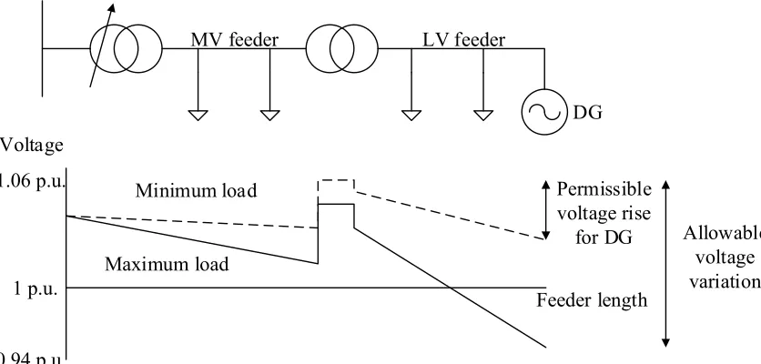
[image:35.595.151.569.514.714.2]

operation [20, 21]. The voltage profile of a radial distribution feeder is shown in Figure 2.1.

Figure 2. 1 Voltage variation down a radial feeder

MV feeder LV feeder

DG

Maximum load

Minimum load Permissible

voltage rise

for DG Allowable voltage variation Voltage

1 p.u. 1.06 p.u.

0.94 p.u.

(36)

14

As indicated in Figure 2.1, the voltage at the starting point of the MV feeder is held

constant by a tap-changing transformer. The voltage drops along the distribution network

due to line impedance and the load on the feeder. The voltage boost in the middle of the

feeder is due to taps of the MV/LV transformer and the voltage drop on the LV feeder is due

to the low voltage loads [22, 23].

When DG is installed by the customer, it is regarded as being directly connected to the

MV network through a step-up transformer. The output power of DG changes the power

flow in the network and causes voltage variation [24]. An example is given for a simple

two-bus radial distribution network as shown in Figure 2.2.

Figure 2. 2 Simple two-bus radial distribution network

The voltage rises at the load busbar caused by DG in per unit (p.u.) can be

approximately calculated by:

2 2

21 2 1

( DG L ) ( DG L )

R P P X Q Q

V V V

V

− + −

(37)

15

where V1 and V2 are the voltages of the primary and load busbars; V is the nominal voltage;

R and X are the circuit resistance and impedance; and PDG-PL2 and QDG-QL2 are the active

and reactive power flowing through the branch. The voltage rise can be controlled by

importing or exporting reactive power from or to the DG. However, in the current practice

of network management by the DNOs, the power factor of DG using rotating generators is

usually required to be set as unity, which means the DG export active power only. This is

due to that it will be difficult for DNO’s to predict the voltage change in the network if DGs

are not operated at unity power factor. This operation strategy may cause significant voltage

violation when the load level changes from high to low.

2.1.1.2 Increase in Network Fault Level

Many types of distribution generation plants use directly connected rotating machines and

these will contribute to the network fault levels. Both induction and synchronous generators

will increase the fault level although their behaviour under sustained fault condition differs.

The rise of fault level depends on the DG capacity and DG location. In urban areas,

the fault level at many of the existing networks is approaching 70% of the switchgear ratings

caused by the additional contribution from dynamic loads [25]. Hence the increase in fault

level by DG connection can cause serious safety issues to the network operation. This can

(38)

16

Furthermore, to increase the short circuit rating of distribution network by upgrading

the switchgear and cables can be extremely expensive and difficult particularly in congested

city substations and cable routes. Current practice to increase the DG penetration without

causing serious fault level rise is to introduce a high impedance, such as high impedance

transformer or reactor between the generator and the network. But this solution is at the

expense of increased power loss and voltage variations at the generator. In recent years,

researchers have been applying fault current limiters (FCLs) and power electronic devices

in the protection with DG penetration [26, 27].

2.1.1.3 Power Quality

Two aspects of power quality are usually considered to be important with DG: 1) transient

voltage variations and 2) harmonic distortion of the network voltage [28]. Depending on the

network circumstance, the installation of DG can either increase or decrease the quality of

the voltage received by other users in the network.

The transient voltage variation is caused during the connection and disconnection of

relatively large DG to the network. The transient voltage variation can be limited by careful

design of DG plant. But for directly connected induction generators on weak networks, the

transient voltage rise can be the limitation on increasing DG penetration rather than

steady-state voltage rise. For synchronous generators, the starting inrush current can be negligible

(39)

17

However, the disconnection of DG at full output may also lead to significant voltage

drops. Incorrectly designed DG plant with power electronic interface to the network may

inject harmonic currents which can lead to unacceptable network voltage distortions.

2.1.2 Technologies Used in Distributed Generation

The technology available for DG varies widely. It generally has the following characteristics.

Firstly, many of the technologies utilise renewable energy resources. The availability of the

different resources varies significantly in areas and efficiency. Secondly, many of the

technologies have been modularized. For instance, technologies like micro-hydro units,

photovoltaic (PV) arrays, wind turbines and fuel cells consist of a number of small modules.

These modules are manufactured in factories and can be installed at the required location in

a very short time comparing to large centralised power stations. Furthermore, each module

unit can function independently despite the status of the other modules, which means the

failure in one module does not affect the other modules. The effect of module failures on the

total available power output is relatively small as compared to a unit failures in large

centralised power stations. Finally, the adding on or relocation of modules is allowed by the

technologies. An important type is the combined heat and power (CHP) generation. This

technology uses various heat generation technologies to supply heat demand and drive

synchronous or induction generators for electricity. Detailed description of several

(40)

18

2.1.2.1 Combined Heat and Power Plants

Combined heat and power is, at present the most significant type of distributed generations.

Generally, the generated electrical power is consumed inside the host premises or industrial

plant of the CHP facility. The heat is either used for the industrial process and/or for space

heating inside the premises or transported for the district heating. The typical overall

efficiency of CHP can be 67% with electrical efficiency of 23% and heat efficiency of 44%

[29]. This would lead to a 35% reduction in the primary energy use compared to electrical

and heat generation from separate power stations and boilers. This further leads to a

reduction in total CO2 emission by over 30%.

The prime movers of CHP units at present predominantly include: gas engine, gas

turbine, fuel cell and domestic boiler system. In the last case, the hot gas firstly drives the

generator to generate electricity through the steam turbine. Afterwards, the gas is passed to

the industrial process or through a heat exchanger for the space heating. The generator,

commonly a synchronous or induction generator, is directly connected to the grid through a

step-up transformer. Due to the capability of reactive power control, synchronous machines

are more preferred than induction machines in the electricity generation of CHP [30, 31].

The grid interface of a fuel cell type of CHP unit is through a power electronic stage

[32]. The fuel cell directly converts fuel energy into heat and electricity without using kinetic

(41)

19

Some small scale domestic CHP units use fuel cell or an external combustion engine

such as Stirling engine to drive a rotary or linear permeant magnet generator. These

small-scale CHP units is connected to the single-phase grid through power electronic interfaces.

The basic configuration of a CHP units with gas turbine is illustrated in Figure 2.3. At

present, most of the CHP units in the distribution network operate in the mode of producing

heat as the main output and electricity as by-product by the current power.

For fuel cell CHP units, the connection to the gird is through a power electronic

interface, as shown in Figure 2.4. This can limit the current contribution to a grid fault [32].

Figure 2. 3 Configuration of a gas turbine CHP [33]

Generator

Coupling Step-up Transformer Gas Turbine

Heat Exchanger

Exhaust Gases

Distribution Network Heat Consumer

Fuel

Compressor

(42)

[image:42.595.271.428.156.402.2]

20

Figure 2. 4 Configuration of fuel cell CHP [34]

2.1.2.2 Renewable Energy Generation

At present, the distribution of DGs using CHP is mainly determined by the local load and

the operation of CHP is generally controlled in response to the energy demands of the heating

scheme. Similarly, the siting of electricity generation using renewable energy source is

determined by the location of the renewable energy source and their output varies with the

availability of the source [35]. For small DGs using renewable energy resources, it is not

cost-effective to provide large energy storage. This is an important difference compared with

(43)

21

2.1.2.2.1 Small-scale Hydro Generation

Hydro generation is a relatively mature technology and the operation of small and medium

sized hydro generating units in parallel with distribution system is well understood [36, 37].

The hydro schemes experience large variation according to availability of the water flow if

significant water storage capacity is not available. This variation is largely affected by the

rainfall, particularly if the catchment is on rocky or shallow soil which lacks vegetation cover

and steep, short streams [38]. Uneven rainfall will lead to a variable hydro resource and it is

interesting to note that the capacity factor for hydro generation in the United Kingdom for

2008 was only some 35%. (Capacity factor is the ratio of annual energy generated to that

which would be generated with the plant operating at the rated output all year).

The power output of a hydro-turbine is given by:

P = Q Hη ρg (2.2)

where P is the output power (W), Q is the flow rate (m3/s), H is the effective head (m), η is

the overall efficiency, ρ is the density of water (1000g/m3) and g is the acceleration due to

gravity (~9.8m/s2_{). Various forms of turbine are used for differing combinations of flow rate}

and head. For small hydro units (<100kW), a cross-flow impulse turbine, where the water

strikes the runner as a sheet rather than a jet, may be used. The typical reasonable efficiencies

(44)

22

Generators commonly used in small-scale hydro scheme are induction or synchronous

machines. Considering the safety of turbine-generator when over-speeding due to the loss of

loads, the squirrel-cage induction generator is more preferred than wound rotor synchronous

machine. Due to the operating characteristic of the turbine to the variable flow rates, the

number of variable speed hydro-generator sets in use is increasing. This requires the use of

power electronic interface for the connection to the distribution network.

2.1.2.2.2 Wind Power Plants

The power developed by a wind turbine extracted from the kinetic energy of the passing

wind is:

3 1

2 p a s

P= C ρ v A (2.3)

where Cp is the power efficiency (a measurement of the effectiveness of the aerodynamic

rotor), P is the output power (W), v is the wind velocity (m/s), As is the swept area of rotor

disk (m2_{) and}_ρ_a_{is the density of air (1250g/m}3_).

As the developed power is proportional to the cube of wind speed, it is very important

to locate the generation in the area of high mean annual wind speed and the availability of

(45)

23

Typically, a 2MW wind turbine has a rotor diameter of 60 to 80 m mounted on a 60 to

90 m high tower. The wind turbine must be designed to withstand large forces during high

winds as the force exerted on the rotor is proportional to the square of the wind speed. The

three-bladed horizontal-axis rotor design gives a good value of power efficiency, which

varies with the relative speed of the rotor and the wind (the tip speed ratio). The maximum

value of Cp in practice is approximately 0.4 to 0.45 [40].

The wind turbine can be operated, in response to the variation of the wind speed, in

fixed or variable speed [41, 42]. For a fixed speed wind turbine, the induction generator is

commonly in use. The schematic representation of a fixed speed wind turbine is shown in

Figure 2.5. The aerodynamic rotor is coupled to the induction generator via a speed

increasing gearbox. The cage rotor induction generator is typically for 690V, 1000 or 1500

rpm. Pedant cables within the tower connect the generator to power factor correction

capacitors and an anti-parallel soft-start unit located in the tower base. The wind turbine is

typically connected into the 11kV or 33kV network in UK through a step-up transformer.

For a variable speed wind turbine, the generator can be either induction or synchronous

generator. The schematics of variable speed wind turbine using induction and synchronous

generators are shown in Figures 2.6 and 2.7. The double fed induction generator (DFIG) uses

a back to back voltage source convertor (B2B VSC) in the rotor circuit. It controls the power

flows when the generator operates above the synchronous speed. If the required speed

operation is in a wide range, the arrangement in Figure 2.7 can be used. The B2B VSC is

(46)

24

The generator can be either induction or synchronous generator and the pulse width

modulation (PWM) control is used on the converter bridges. The variable speed operation

[image:46.595.253.442.273.452.2]

gives two main advantages: 1) reducing the mechanical loads and 2) smoothing output power.

Figure 2. 5 Fixed speed induction generator wind turbine [43]

[image:46.595.259.437.541.717.2]

(47)

[image:47.595.250.445.181.359.2]

25

Figure 2. 7 Figure 2.7 Full power converter wind turbine [43]

2.1.2.2.3 Solar Photovoltaic Generation

Photovoltaic generation is a well-established technology with a number of major

manufactures producing related equipment. The physics of photovoltaic energy conversion

has been described by a number of authors [44-46]. Its main application was off-grid for

high value and small electrical load that were far from the nearest distribution network for

many years in the past. In the recent years, stimulated by support through feed-in tariffs its

use as grid-connected distributed generation has increases rapidly particularly in Germany

and Spain [47, 48]. The interests of PV generation in Europe is focused on smaller

(48)

26

These small PV installations are connected directly at customers’ premises and so to

the low voltage distribution network. This form of generation is distributed largely in

residential and commercial customers. The schematic representation of a small PV

generation connected to the grid is shown in Figure 2.8. The inverter typically consists of :1)

a maximum power point tracking (MPPT) circuit, 2) an energy storage element, 3) a dc to

dc converter to increase the voltage, 4) a dc-ac convert stage, 5) an isolation transformer and

6) an output filter. Usually PV inverters operate at unit power factor and have a very limited

effect on the network voltage [49, 50].

(49)

27

2.1.3 Grid Regulation and Standards Regarding DG

Installation

Embedded generators above 11kVA in MV or LV networks are governed by Engineering

Recommendation G59 (Issue 3, 2013) [52, 53]. The main schemes used in the UK regarding

the aspects mentioned in Section 2.1.1 are as follows.

Voltage limits

Where the generating plant is remote from a network voltage control point, a voltage

range of ±10% of the declared voltage is applied at the connection point. The step voltage

change caused by the connection and disconnection of generating plant from the distribution

system is subject to a typical limit of ±3% for infrequent planned switching events and ±10%

for unplanned outages.

Power quality

The connection and operation of generating plant may cause a distortion of the

distribution system voltage waveform resulting in voltage fluctuations, harmonics or phase

voltage unbalance. The limits on the low order harmonic distortion are set as shown in Table

(50)

[image:50.595.191.479.186.428.2]

28

Table 2. 1 Limits for harmonic emission [53]

Harmonic order Maximum permissible harmonic current

n A

Odd harmonics

3 2.3

5 1.4

7 0.77

9 0.4

11 0.33

13 0.21

15≤n≤39 0.15x8/n

Even harmonics

2 1.08

4 0.43

6 0.3

8≤n≤40 0.23x8/n

Protection setting

In order to avoid unnecessary disconnection of generating plant during distribution

network faults or switching events and the consequent disruption to generators and

(51)

29

Table 2. 2 Settings for long-term parallel operation [53]

Protection Function

Small Power Plant①

Medium Power Plant②

LV③_Protection _HV④_Protection

Trip Setting Trip Delay Time (s) Trip Setting Trip Delay Time (s) Trip

Setting Trip Delay Time (s)

U/V stage 1 Vϕ-n⑤

-13% 2.5 Vϕ-ϕ

⑥

-13% 2.5 Vϕ-ϕ⑥

-13% 2.5

U/V stage 2 Vϕ-n⑤

-20% 0.5

Vϕ-ϕ⑥

-20% 0.5

O/V stage 1 Vϕ-n⑤

+14% 1

Vϕ-ϕ⑥

+10% 1 Vϕ-ϕ⑥

-13% 1

O/V stage 2 Vϕ-n⑤

+19% 0.5

Vϕ-ϕ⑥

+13% 0.5

U/f stage 1 47.5Hz 20 47.5Hz 20 47.5Hz 20

U/f stage 2 47Hz 0.5 47Hz 0.5 47Hz 0.5

O/f stage 1 51.5Hz 90 51.5Hz 90

51.5Hz 0.5

O/f stage 2 52Hz 0.5 52Hz 0.5

Loss of Mains

(Vector Shift) K1⑦ x 6 degrees K1⑦ x 6 degrees Inter-tripping expected Loss of Mains

(Rate of Change

of Frequency) K2

⑧_{x 0.125 Hz/s} _K₂⑧_{x 0.125 Hz/s} Inter-tripping

[image:51.595.114.555.190.527.2]

expected

Table 2. 3 Settings for infrequent short-term parallel operation [53]

Protection Function

Small Power Plant①

LV③_Protection _HV④_Protection

Trip Setting Time (s) Trip Setting Time (s)

U/V stage 1 Vϕ-n⑤ -10% 0.5 Vϕ-ϕ⑥ -6% 0.5

O/V stage 1 Vϕ-n⑤ +14% 0.5 Vϕ-ϕ⑥ +6% 0.5

U/f stage 1 49.5Hz 0.5 49.5Hz 0.5

Network fault analysis with increased distributed generation penetration and evaluation of solutions to issues caused by distributed generation

warwick.ac.uk/lib-publications

Network Fault Analysis with Increased

Distributed Generation Penetration and

Evaluation of Solutions to Issues

Caused by Distributed Generation

Han Qin

A Thesis Submitted for the Degree of

Doctor of Philosophy

School of Engineering

The University of Warwick

Contents

List of Figures

List of Tables

Declaration

Acknowledgement

Abstract

Nomenclature

Introduction

1

1.1

History of Electrical Power System

1.2

Brief Introduction to Distribution Network

1.3

Brief Introduction to Distributed Generation

1.4

Research Objectives and Contributions

1.5

Outlines of the Thesis

Literature Review

2

2.1 Review of Distributed Generation

2.1.1

Technical Impacts of Distributed Generation on the

Distribution Network

2.1.1.1

Network Voltage Changes

2.1.1.2

Increase in Network Fault Level

2.1.1.3

Power Quality

2.1.2 Technologies Used in Distributed Generation

2.1.2.1

Combined Heat and Power Plants

2.1.2.2

Renewable Energy Generation

2.1.2.2.1

Small-scale Hydro Generation

2.1.2.2.2

Wind Power Plants

2.1.2.2.3

Solar Photovoltaic Generation

2.1.3 Grid Regulation and Standards Regarding DG

Installation