Machine learning classification tool for innovation projects

(1)

Machine learning classification tool for

innovation projects

Master thesis Business Administration

Author: T. Oord (1870564) Date: 24/06/2019

Supervisors: dr. M. de Visser

dr. R.P.A. Loohuis MBA

(2)

II

Abstract

(3)

III

1 Introduction

1.1 Background

In 1934 Schumpeter emphasizes the importance of innovations and technology in economic progresses and he became the founder of economics of innovation (Schumpeter J. A., 1934). Nowadays innovation is very important for the continuity of a company due to rapid technological changes. Investments are needed to achieve innovation. Most investors want to obtain the highest return for the lowest amount of risk (Brentani, 2004). However, there is a trade-off between the amount of risk and return on investment. A higher risk is generally associated with a higher return. Therefore, a manager needs to determine the amount of risk, and the potential return an innovation could gain in the future. A well-balanced innovation portfolio is critical to ensure a company’s continuity (Cooper, Edgett, & Kleinschmidt, 1999). A business list of active new products and new R&D projects have to be constantly updated and revised to ensure the innovation portfolio is well-balanced. Existing projects may be accelerated or aborted, and resources need to be allocated or reallocated to the active and most prospective projects. High innovative businesses can become too risky, while low innovative organizations may become obsolete (Levinthal & March, 1993).

To find out if the innovation portfolio is well-balanced organisations should classify their innovation projects. Organizations produce a lot of semi-structured data of innovation projects that could be used for this classification. But, exploiting these data for portfolio management is hard and time consuming, because data needs to be organized and classified. Additionally, many typologies in the literature of the economics of innovation overlap with each other or are inconsistent (Coccia, 2006). This makes company’s innovation portfolios hard to compare with each other. Even in academic research this literature is hard to compare because of overlapping typologies and definitions (Coccia, 2006).

Recent developments in Machine Learning, especially Natural Language Processing (NLP) are promising in classifying innovation portfolio data more effective and efficiently. De Visser et. al. (2017) were the first to investigate machine learning-based analysis of innovation projects and showed great opportunities on improving innovation portfolio management.

1.2 Goal and research questions

In this thesis the potential of automatic classification of project descriptions will be investigated and tested. The aim of this research is to develop a machine-learning tool for automatic classifying innovation descriptions into useful innovation taxonomies. Subsequently, the automatic classified data will be visualized, and the potential of this application will be discussed. To achieve this research goal the following research question has been formulated:

How can innovation descriptions automatically be classified using a machine learning approach, and which conclusions can be drawn of the sample’s portfolio trends?

In order to give the master thesis a better structure, several sub-questions were added: Q1: Which innovation typologies can be used for measuring innovation portfolios?

Q2: How can the training data be labelled with a high inter-rater-agreement in order to attain a reliable training set?

Q3: Which classifiers are best performing?

(6)

2

1.3 Research method

This research will solve the research problem by answering the research questions. The research consists of the following parts: a theoretical part; an empirical part; an analytical part; and a concluding part. The theoretical part consists of two literature reviews which are addressed in chapter 2. The first part (2A) answers research question Q1. This is done by reviewing the relevant academic literature and provides a theoretical base of innovation classification. The second section focusses on getting more knowledge about the labelling techniques and the theory on machine-learning. This will be used to answer research question 2 in the empirical part of the research.

The empirical part will be addressed in chapter 3. In this part, the innovation description from the dataset will be used. The innovation typologies of the theoretical part and the theory of labelling techniques of chapter 2 will be applied on the innovation descriptions. Research question 2 will be answered in this part. Subsequently, the labelled data will be used to perform the machine-learning process. These results will be given in the analytical part.

(7)

3

2 A: Literature study: Innovation

In order to develop a machine learning tool for innovation project descriptions it needs to be understood what an innovation portfolio is, and which innovation typologies are used in academic literature. Subsequently, in part 2B, literature on different labelling techniques will be discussed as well as the literature on machine learning. A thematic literature review is applied from reviewing the key studies on these topics.

2.1 Innovation

Economics of innovation is about the forces that drive innovation, hinder it and effects industry, market or economy. Schumpeter (1942) coined the term ‘creative destruction’ which he described as: “the process of industrial mutation that incessantly revolutionizes the economic structure from within, incessantly destroying the old one, incessantly creating a new one" (Schumpeter J. , 1942, p. 81). This aspect of innovation clearly distinguishes innovation from invention, because an innovation creates some form of economic value, where an invention can stick to an idea only.

After Schumpter coined the term ‘creative destruction’, the diffusion theory described the process by which innovations are adopted over time (Rogers, 1962). Later, many typologies were distinguished by many researchers. In a literature review on the similarity and/or heterogeneity of typologies of innovation present in the economic fields, Coccia (2006) emphasizes that “economic literature uses different names to indicate the same type of technical change and innovation, and the same name for different types of innovation” (Coccia, 2006, p. 8). This problem needs attention, before applying it to machine learning purposes.

2.2 Portfolio management

Cooper (1999, p. 335) defines innovation portfolio management as follows:

“Portfolio management is a dynamic decision process, whereby a business’s list of active new product (and R&D) projects is constantly updated and revised. In this process, new projects are evaluated, selected, and prioritized; existing projects may be accelerated, killed, or deprioritized; and resources are allocated and reallocated to the active projects.”

Brasil and Eggers (2019) define portfolio management as a source of competitive advantage that supports organizational renewal. In the literature of new product development (NPD), Kleinschmidt and Cooper (1991) state that a well-balanced innovation portfolio is vital to ensure a company’s continuity. This balance implies the allocation of resources to innovation projects to achieve product development goals. Companies need to recognize future opportunities through the development of new products (Danneels, 2002). The product innovations can contribute to firm renewal and thus expansion of organizational competences over time. On the other hand, companies need to determine whether their current product portfolio fits with their strategic management and organization (Macmillian, Hambrick, & Day, 1982).

(8)

4

Google’s cofounder Lay Page told Fortune magazine that his company also strives to achieve this 70-20-10 balance (Page, 2008). On the contrary, the distribution of total return is the inverse of the resource allocation ratio. As a matter of fact, the ratio is not applicable to all companies. For instance, industry, ambition and the stage of a company’s development are factors that influence this ratio too.

In order to support portfolio decision making, several new product portfolio methods are used. Ranging from financial models (Net present value, expected commercial value, decision tree) as well as non-financial models (Strategic buckets, scoring model and bubble diagram) (Cooper, Edgett, & Kleinschmidt, 1999).

Innovation portfolio is essential to have a clear overview of current projects in order to evaluate and adjust the projects if needed. A business list of active new products and new R&D projects have to be constantly classified, updated and revised to ensure the innovation portfolio is well-balanced. This is a time-consuming process and difficult because of the many typologies used in literature. Automatic classification may decrease the time significantly. However, a clarification of the different innovation typologies is needed first. The next sections will discuss the different innovation typologies and underlying dimensions in literature.

2.3 Types of innovation

In a report from Eurostat and the Organization for Economic Co-operation and Development (OECD) a framework is provided what enables innovation management. They define innovation as: “a new or improved product or process (or combination thereof) that differs significantly from the unit’s previous products or processes and that has been made available to potential users (product) or brought into use by the unit (process)” (OECD, 2018, p. 22). They distinguish two main types of innovation:

• “Product innovation is a new or improved good or service that differs significantly from the firm’s previous goods or services and that has been introduced on the market” (OECD, 2018, p. 21).

• “Business process innovation is a new or improved business process for one or more business functions that differs significantly from the firm’s previous business processes and that has been brought into use by the firm” (OECD, 2018, p. 21).

2.4 Customer level and firm level

(9)

5

2.5 Degree of novelty

Besides the differences between the type of innovation and the level of innovation, great distinction is made between the innovation’s degree of novelty. This section will describe the different typologies used in literature in order to find the underlying dimensions.

2.5.1 Transilience map

In 1985 Abernathy and Clark (1985) developed a model called ‘the transilience’ map in order to predict a firm’s future strategy on innovation and change. They map four different types of segments by linking the following dimensions:

1. Novelty of technology / production; how new technology and manufacturing activities are being organized

2. Novelty of market / customer; activities needed by the firm to service new markets and customers

This results in the segments: Architectural, Niche Creation, Regular and Revolutionary. Each quadrant in the map represents a different kind of innovation and tends to be associated with a different kind of competitive environment, as shown in Figure 1 (Abernathy & Clark, 1985). The dimensions can be used in firm- and customer perspective.

2.5.2 Newness to the market and newness to the firm

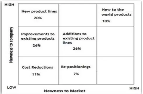
Booz, Allen and Hamilton (1982) categorize

new products into a six-stage classification scheme as shown in Figure 2. The concept was based on two dimensions:

1. Newness to the company 2. Newness to the marketplace For example, ‘new-to-the world products’ are new for the company and the customer. Whereas the novelty for ‘cost reductions’ are low on both axes. Both levels (firm perspective and customer perspective) are used in this typology. Most innovation typologies are built upon the typology of Booz, Allen and Hamilton.

2.5.3 Incremental and radical innovations

[image:9.595.279.523.165.325.2]

Freeman et. al. (1982) distinguished two different types of technical change. Incremental or sustaining innovations occur almost continuously and in any industry. These innovations go along with quality improvements of existing products, services or processes. On the other hand, radical innovations have a bigger technological impact. However, radical innovations are discontinuous events and occur less common than incremental innovations. Incremental innovations go along with less risk compared with

Figure 1 Transilience map Abernathy and Clark (1985)

[image:9.595.279.525.463.624.2]

(10)

6

radical innovations. But the economic impact of radical innovations is greater than incremental innovations (Freeman, 1982).

2.5.4 Architectural and modular innovations

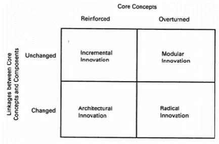
Besides the literature of incremental and radical innovation some literature states that this categorization is incomplete and potentially misleading (Henderson & Clark, 1990). For this reason, Henderson and Clark (1990) coined the term ‘Architectural innovation’ and ‘Modular innovation’. Architectural innovations are innovations that change the architecture of a product (to enter a new market) without changing its components (technology). On the other hand, a modular innovation replaces a component without changing the architecture of a product. This model is shown in Figure 3.

2.5.5 Disruptive innovations

The term disruptive innovation is first addressed by Christensen (1997). Generally, a disruptive innovation is a product or service designed for a new set of customers in an existing market and eventually disrupts the existing market (Christensen, 1997). First the existing product is suitable for only a small population and after transformation the product is suitable for a larger population.

2.5.6 Exploitation and exploration

The distinction between explorative and exploitative innovation was first made by March (1991). Exploration includes things like search, variation, risk taking and experimentation. Returns are systematically less certain, and firms may not have complete information of all possible opportunities (Benner & Tushman, 2003). On the other hand, exploitation focusses on the development and refinement of existing products or developments for current customers. The returns on exploitation are more certain and closer in time (Trimble & Govindarajan, 2010; March, 1991). March (1991) considers the relation between the exploration of new possibilities and the exploitation of old certainties in organizational learning. Both are important but organizations make explicit and implicit choices between them in order to allocate resources. Understanding these choices is complicated because the returns from both options vary with respect to their expected values and their variability, timing and their distribution within the organization (March, 1991). From a market learning perspective, market exploration refers to the search and pursuit of completely new knowledge and skills outside the firm’s current product market and market exploitation emphasizes the use and refinement of existing knowledge and skills in the current product market (Zhang, Wu, & Cui, 2015).

[image:10.595.305.522.136.278.2]

Often, firms focus more on either exploration or exploitation which results in bad performance in the long term. Organizations that focus exclusively on exploitation may become obsolete (Levinthal & March, 1993). Alternately, organizations focussing only on exploration may not take the benefits of the investments made. The ability of an organization to both exploit and explore is called ‘organizational ambidexterity’ (Birkinshaw & Gibson, 2004; Tushman & O'Reilly, 1996).

(11)

7

2.6 Drivers of innovation

The drivers of innovation are the major forces behind a firm’s innovation (Strecker, 2009). Gatignon and Xuereb (1997) show that a firm’s strategic orientation (market, technology or competitor) on new product development is essential for the performance of a firm. Market-based or market pull innovations are innovations that result from market needs. Technology-based or technology push innovations are innovations that start within the company’s R&D department and subsequently find a demand in a market. Competitive orientation focusses on observing, analysing and responding to competitors’ new products (Gatignon & Xuereb, Strategic orientation of the firm new product performance, 1997). Dosi (1988) states that an incremental innovation is mostly a market pull innovation, while a radical innovation is often a technology push innovation (Dosi, 1988).

2.7 Innovation and economic benefits

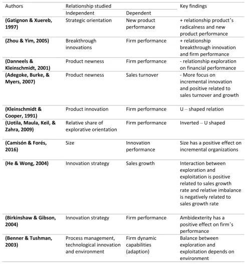
In previous sections various types of innovations in literature are discussed. The relation between these typologies and economic benefits will be discussed in this section and are summarized in Table 1. Despite the fact that these effects differ widely, and empirical research is still scarce, some literature is found on a positive relation between the degree of novelty and the economic benefits ( (Gatignon & Xuereb, 1997; Zhou & Yim, 2005). On the other hand, Danneels and Kleinschmidt (2001) found a negative relationship between innovativeness and product performance. In research on SMEs in the United Kingdom they found that SMEs tend to focus more on incremental than radical innovations and that this focus is related to growth in sales turnover (Adegoke, Burke, & Myers, 2007). Kleinschmidt and Cooper (1991) found a U-shaped relationship between product innovativeness and firm performance. Which means that high and low innovative products are more likely to be more successful than those in between. On the other hand, a longitudinal panel research, covering data from 1989 – 2004 for 279 manufacturing firms in the 1989 S&P 500 index, found an inverted-U shaped relationship between a firm’s relative exploration orientation and its financial performance (Uotila, Maula, Keil, & Zahra, 2009). It appears to be there is not a consistent outcome in literature so far.

Uotila et. al. (2009) also found that the relationship between the relative amount of exploration orientation and financial performance is moderated by the research and development intensity of the industry in which firms operate. Camisón and Forés (2016) state that incremental innovation performance is positively affected by internal knowledge creation and absorptive capabilities and size has a direct positive effect on incremental innovation performance.

In a study on ambidexterity and firm performance they found evidence that (1) interaction between explorative and exploitative innovation strategies is positively related to sales growth rate, and (2) the relative imbalance between explorative and exploitative innovation strategies is negatively related to sales growth rate (He & Wong, 2004). Additionally, Birkinshaw and Gibson (2004) found empirical evidence that ambidexterity has a positive effect on a firm’s performance. However, Benner and Tushman (2003) state that the balance between exploration and exploitation also depends on the environment an organization operates in.

(12)

[image:12.595.67.557.124.651.2]

8 Table 1 Research on innovation strategy and performance

Authors Relationship studied Key findings

Independent Dependent

(Gatignon & Xuereb, 1997)

Strategic orientation New product performance

+ relationship product’s radicalness and new product performance

(Zhou & Yim, 2005) Breakthrough innovations

Firm performance + relationship

breakthrough innovation and firm performance

(Danneels &

Kleinschmidt, 2001)

Product newness Firm performance - relationship exploration on financial performance

(Adegoke, Burke, & Myers, 2007)

Product newness Sales turnover - More focus on incremental innovation and positive related to sales turnover and growth

(Kleinschmidt & Cooper, 1991)

Product innovation Firm performance U – shaped relation

(Uotila, Maula, Keil, & Zahra, 2009)

Relative share of explorative orientation

Firm performance Inverted – U shaped

(Camisón & Forés, 2016)

Size Innovation

performance

Size has a positive effect on incremental organizations

(He & Wong, 2004) Innovation strategy Sales growth Interaction between

exploration and exploitation is positive related to sales growth rate and relative imbalance is negatively related to sales growth rate

(Birkinshaw & Gibson, 2004)

Innovation strategy Firm performance Ambidexterity has a positive effect on firm’s performance

(Benner & Tushman, 2003)

Process management, technological innovation and environment

Firm dynamic capabilities (adaption)

Balance between exploration and

(13)

9

2.8 Conclusion chapter 2A

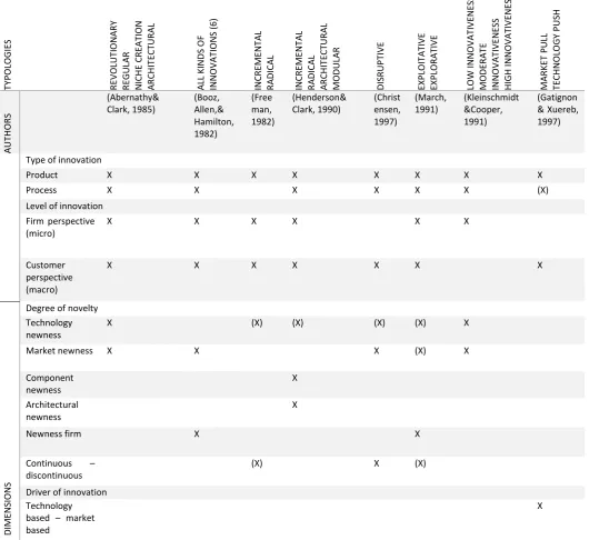
[image:13.595.36.567.238.724.2]

Despite many typologies have a high level of abstraction, Table 2 implicates a structured overview of the relevant typologies with underlying dimensions. Some typologies use two dimensions, while others use a mixture. For example, the typology of March does not use contrary measurements, which makes it harder to operationalize.

Table 2 Innovation typologies and underlying dimensions

TY PO LO G IE S R EV O LUT IO N A R Y R EG UL A R N ICH E CR EA TI O N A R CH IT EC TURA L A LL KIN DS O F IN N O V A TIO N S ( 6) IN CR EME N TA L R A DICA L IN CR EME N TA L R A DICA L A R CH IT EC TURA L MO DU LA R DIS R UPT IV E EXP LO IT A TI V E EXP LO R A TIV E LO W IN N O V A TI V EN ES S MO DE R A TE IN N O V A TIV EN ES S H IG H IN N O V A TIV EN ES S MA R KE T PUL L TE CH N O LO G Y P US H A UT H O R S (Abernathy& Clark, 1985) (Booz, Allen,& Hamilton, 1982) (Free man, 1982) (Henderson& Clark, 1990) (Christ ensen, 1997) (March, 1991) (Kleinschmidt &Cooper, 1991) (Gatignon & Xuereb, 1997)

Type of innovation

Product X X X X X X X X

Process X X X X X X (X)

Level of innovation Firm perspective (micro)

X X X X X X

Customer perspective (macro)

X X X X X X X

DIME

N

SIO

N

S

Degree of novelty Technology newness

X (X) (X) (X) (X) X

Market newness X X X (X) X

Component newness X Architectural newness X

Newness firm X X

Continuous –

discontinuous

(X) X (X)

Driver of innovation Technology based – market based

(14)

10

2 B: Literature study, Machine-learning

2.9 Semi-structured data

Over the past decades organizations have produced large amounts of semi-structured data due to the introduction of information systems (de Visser, Miao, Englebienne, Sools, & Visscher, 2017). Information systems produce data like project descriptions and progress reports. This data has the potential to be used in portfolio management and associated innovation research.

As mentioned before, a well-balanced portfolio is critical to ensure the continuity of a company. From a practical perspective this data can give managers useful insight in order to make conclusions of their innovation portfolio and help them to make decisions on their innovation strategy. From an academic perspective this existing data could be used to do research on the effects of types of innovation. Instead of gathering new data, the use of existing data can simplify research.

The data mentioned is most of the time not structured and largely textual and it is hard to extract information from it. Besides manual analysis could be time-consuming, unreliable and inconsistent. Nowadays there are new options to make use of this data more efficiently by using artificial intelligence and big data techniques. This potential will be described in the next section.

2.10 Machine-learning

Machine learning is part of artificial intelligence and deals with programming computers to optimize a performance criterion using training data or experience. It is used in cases where you cannot directly use an algorithm to solve a problem but need training data or experience (Alpaydin, 2010). Natural Language Processing (NLP) is also part of artificial intelligence and deals with the analysis of textual data using machine learning. Machine learning can be split up into supervised learning and unsupervised learning.

Most of the practical machine learning problems use supervised learning. In supervised learning you have input variables (x) and output variable (y) and an algorithm to learn the mapping function input to output. The goal is to predict the output variables for new input data. However, the training data needs to be labelled in order to train the classifier. The amount of required labelled training data depends on many variables like the complexity of the problem, learning algorithms, number of classes and the quality of the data. The training will stop when the algorithm achieves an acceptable level of performance. Supervised learning problems can be grouped into classification and regression. A classification problem has a category as output variable and a regression problem deals with real values as output variable.

Unsupervised learning has no corresponding output variables and has only input data. The goal is to model the underlying structure in order to learn more about the data. There is no ‘correct answer’

and no teacher to train the algorithm. Unsupervised learning problems can be grouped into clustering and association. A clustering problem is when you are looking for inherent groupings in data. Association problems are when you want to discover rules between variables in large databases. Unsupervised learning requires more input data than super-vised learning and is mostly useful in finding out whether information exists in the dataset. Semi-supervised learning sits in between both and uses large amount of input data, where only some of the training data is labelled.

(15)

11

De Visser et al. (2017) were the first to investigate machine learning-based analysis of innovation project descriptions in firms. They found that it is possible to achieve a high level of accuracy. But training based on expert judgment is required to reach high accuracy and thus time consuming. This is a steppingstone towards more complex analyses and larger amounts of projects descriptions. Roelofs (2018) compared different supervised and semi-supervised classifiers in order to test automatic classification of innovation portfolio descriptions. The most accurate results were achieved by a naïve Bayes classifier, which outperformed human classification. But they found that the

inter-rater agreement between inter-raters was very low with a Cohen’s Kappa of only 0.15 for the exploration –

exploitation typologies (Roelofs, 2018). They suggested using expert judgements for labelling and semi-supervised learning did not give notable increase in performance. This research draws on their research and contributes to the research on machine learning-based classification of innovation projects. Theory on inter-rater agreement will be discussed in the next section.

2.11 Labelling training sample

2.11.1 Inter-rater agreement and inter-rater reliability

In order to train a machine-learning classifier in supervised machine-learning, a reliable labelled training dataset is required (Alpaydin, 2010). To label instances manually requires a reliable inter-rater agreement between coders. The inter-rater agreement is often measured as the percentage of agreement between coders. However, the inter-rater agreement doesn’t test the reliability. This is often measured as the Cohen’s Kappa, which determines the extent to which judgements are reproducible, i.e., reliable (Cohen, 1960). This is interpretable as “the proportion of joint judgements in which there is an agreement, after change agreement is excluded” (Cohen, 1960, p. 46). A Cohen’s Kappa between < 0.2 is interpreted as a poor agreement, 0.2 – 0.4 a fair agreement, 0.4 – 0.6 a moderate agreement, 0.6 – 0.8 a substantial agreement and 0.8 – 1 is an almost perfect agreement (Landis & Koch, 1977).

2.11.2 Labelling methods

Many approaches and tools can be used for labelling data. Internal labelling approaches results in high accuracy and the ability to track the process. But it takes a lot of time. Approaches like outsourcing (requirement of temporary employees) and crowdsourcing (cooperation with platforms) are less time consuming but have a quality risk and are expensive (Datascience, 2018).

(16)

12

3 Methodology

In this chapter the methodology used in this research is described. In Figure 4 a flowchart of this research is presented.

3.1 Data

The dataset used in this project includes 4691 anonymized project descriptions from 440 manufacturing firms in a time frame of five years. The project descriptions describe innovative projects and are written for innovation grant applications by a European consultancy firm. Another three years of data was collected with the intention to extend the dataset for this research. However, the structure of the new data was somewhat different than the existing dataset. For this reason, within the timeframe of this research, there was not enough time and resources to restructure and anonymize this dataset.

There are several reasons why the data is not totally representative of firms in general. First, because of the grant application, the innovation descriptions are somewhat exaggerated in terms of innovativeness. Secondly, not all firms may outsource their grant application at the relevant company or will only outsource a small piece of the innovation grant applications. Despite that, the diversity of companies and the amount of project descriptions make this dataset interesting to use.

The descriptions that are used in this project contain approximately 250 words. These descriptions usually describe the situation, the goal and technical characteristics of the project. But the nature of the descriptions is slightly different from each other. For example, some descriptions carefully describe the market situation while others emphasize on the technical aspects of the innovation. Besides the innovation descriptions, there are several variables like the estimated hours work, start and end date and categorization of the project (product, process, software). Only the textual descriptions are used to train the classifier. The date and projects hours are used for trend analysis at a later stage of this project.

3.1.1 Data selection

[image:16.595.289.526.144.479.2]

Not every project description in the dataset is unique because some long-running projects were updated for resubmission. The dataset was condensed by Roelofs (2018) and is used in this project for training the machine-learning model. This dataset contains only unique project descriptions, in which information from new descriptions was added to the existing one. This result in a dataset of 2097 unique project descriptions. The samples for the label sessions were taken randomly from the

(17)

13

condensed dataset. However, not all descriptions were labelled. This will be discussed later in this chapter. For the prediction and visualization, the total dataset of 4691 project descriptions was used.

3.2 Typologies

The innovation typologies and underlying dimensions are described in chapter 2A. All underlying dimensions were applied on the data in order to evaluate applicability on the relevant data. The typology of March (1991) was used without using dimensions, because the literature has not provided clear underlying dimensions and most research only refer to March’s definition. Finally, the typology ‘business to business’ and ‘business to consumer’ (b2b-b2c) was applied on the data, because during the label session this typology seemed most appropriate for this data.

3.2.1 Label sessions

In order to achieve a high inter-rater-reliability several coding sessions were conducted. The dimensions and typologies have been tried on the data with several methods. This will be discussed in the following sections.

3.2.1.1 First label session

In the first label session the two coders individually labelled 31 instances on explorative or exploitative innovation, based on the definition of March. This resulted in a low inter-rater agreement because rater B labelled all instances as exploration. This was because all instances could be seen as ‘exploring new possibilities’. This suggest that the raters tend to label an instance directly into a category, as soon as one of the aspects that are mentioned in the author’s definition are met. March’s definition of both typologies is not always the opposite which makes it harder to classify. This was also supported by Popadiuk and Bido (2016) who concluded that the idea of exploration and exploitation is complex and cannot simply elaborate a definition in a few words. Another reason for the low score was the perspective from which the rater should label the instances. Rater A focussed on the product described in the description, while rater B focussed on the organizational aspects. In conclusion, labelling based on just the author’s definition results in different interpretations between coders and thus a low rater-reliability. A more delimited definition was needed in order to increase the inter-rater-agreement.

3.2.1.2 Second label session

In order to make the labelling session more structured, the definitions of the typologies were clarified by using a code scheme (as described in chapter 2.11). In addition, a 5-point scale was used to make a more robust choice. The code scheme was tested using two measurements which were based on the study of Kleinschmidt and Cooper (1991) and adjusted by Ericson and Kastenson (2011). Measurements were chosen by a 5-point scale. For the first typology <6 points are incremental innovation and >6 are radical. For the second typology <6 is exploitation/incremental and >6 is exploration/radical. The main purpose of the scale was to give the rater a better understanding in labelling.

(18)

14

3.2.1.3 Third label session

In the third and last label session the code scheme was adapted based on the results of the previous label sessions. 10 instances were labelled separately by both coders for all before mentioned dimensions and typologies. The code scheme adapted to previous label session can be found in appendix A. The dimensions and typologies for the final labelled dataset were based on the inter-rater-agreement and the rater’s opinion. The inter-rater-agreements and Cohen’s Kappa are shown in Table 3.

Table 3 Inter-rater-agreement

The first four dimensions have a high inter-rater-agreement, but the Cohen’s Kappa performed very low. This is because almost all descriptions were labelled as one class. For example, nine of the ten instances, for market newness (customer perspective) were classified as ‘existing market’. The raters conclude that it is hard to classify the market newness and technology newness dimensions without having / using prior market- or technology knowledge. For this reason, it has been decided to exclude the dimensions technology newness and market newness from both perspectives. This resulted in five dimensions and typologies that will be used to classify the final sample.

3.2.2 Final sample

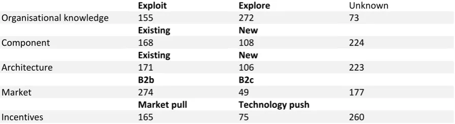
[image:18.595.76.524.604.726.2]

After the label sessions, the code scheme was used as a baseline for the five selected dimensions and typologies. A sample of 500 randomized descriptions were labelled for the relevant dimensions and typologies. Five datasets were created as shown in Table 4.

Table 4 manually labelled datasets

Exploit Explore Unknown

Organisational knowledge 155 272 73

Existing New

Component 168 108 224

Existing New

Architecture 171 106 223

B2b B2c

Market 274 49 177

Market pull Technology push

Incentives 165 75 260

Some descriptions are hard to classify for a dimension due to the lack of information. It has been decided to exclude cases from the sample that are hard to classify. For example, some cases do not

Dimension / typology

Inter-rater-agreement

Cohen’s Kappa

Technology newness (customer perspective) 0.6 0.04

Market newness (customer perspective) 0.9 0

Technology newness (firm perspective) 0.5 -0.3

Market newness (firm perspective) 0.9 0

Component newness (product level) 0.7 0.34

Architectural newness (product level) 0.6 0.17

Exploitation – exploration (innovation process) 0.6 0.2

Market pull – technology push (incentive) 0.9 0.73

(19)

15

describe technical aspects of the product. This makes it hard to classify the component and architecture dimensions. Excluding these cases creates a more powerful training set. However, it potentially influences the representation of the population. A training with an ‘unknown’ class will also be performed. Also, a sixth dataset was created using the already existing product, process, software class. This dataset will be used to compare the classifier’s performance with the size of the training sets. Thereby, this label was already given in the dataset and is not affected by the inter-rater reliability.

3.3 Machine-learning

Before the classifiers can be used, several operations need to be processed on forehand. In this project five datasets are created for the relevant labels. In addition, an extra dataset for each class was created with the ‘unknown’ label and a dataset for the class ‘product, process and software’ was created. Every dataset is split into an 80% training set and a 20% test set. The training set will be used to train the classifier and the test set will be used to test the accuracy of the classifier. Notepad++ is used to create the dataset in ‘.Arff’ format which is used by Weka. The next pre-processing steps will be discussed in the next section and are performed by the machine-learning program ‘Weka’.

3.3.1 Pre-processing

Before the data can be used for training the classifier, the data needs to be pre-processed. This is important because of getting rid of less useful information and transforming the text in something the algorithm can digest. First, tokenization is used to convert the string of text into separate words (called tokens). Subsequently, punctuations were removed, and upper-case tokens are transformed into lower case tokens. Then, stop words were removed by using a combination of several Dutch stop word lists. These stop words (e.g. ‘and’, ‘or’) are meaningless words that could influence the classifier in a wrong way. Finally, tokens were transformed to one base-word by using ‘stemming’ (e.g. ‘performs’, ‘performed’, ‘performing’ becomes ‘perform’). The pre-processing settings used in Weka are shown in Appendix B.

3.3.2 Feature selection

After the data was pre-processed features (or attributes) were extracted. These features are the variables that are relevant to the predictive modelling problem. Not every feature will be used for classification. There are several methods for feature selection and the different methods influence the final accuracy of the classifier. The theory-based method uses several features derived from theory as used in the research of De Visser et. al. (2017). Another method is based on high frequency keywords, were the most common words are used as features (Rajaraman & Ullman, 2011). Another widely used method is the TF-IDF approach, measuring the importance of a word reflected to the document (Rajaraman & Ullman, 2011). Finally, the high information gain keywords method calculates how common a word occurs in a particular category compared to eachother (Perkins, 2014). In a paper on machine learning-based classification of innovation descriptions de Visser et. al. (2017) the best results were achieved with the info gain feature selection method. Additionally, Roelofs (2018) used this feature selection method as well. In this project the TF-IDF method is used, as well as a combination of the TF-IDF method and the info gain method. Both methods are used to test the results between those methods on classifier performance.

3.3.3 Imbalanced classes

(20)

16

project all classes are imbalanced. To handle this imbalanced classes several methods are used. First, Synthetic Minority Over-sampling Technique (SMOTE) was used to create synthetic data for the minority class (Chawla, Bowyer, Hall, & Kegelmeyer, 2002). Accordingly, this technique increases the accuracy level of the classifier. However, all synthetic data were correctly classified, while it did not increase the performance of the classifier on the original data. This concludes that this technique didn’t work out for this dataset. Another method is called ‘cost-sensitive learning’. Different cost factors will be applied on the minority’s false-positives or false-negatives what will lead to a better performance (Kao & Poteet, 2007). Cost-sensitive factors from 1 to 10 were conducted, with no big difference in the confusion matrix. Finally, the dataset could be balanced by leaving data of the majority sample behind. This decreases the sample size, but it was the only method that reached a balanced and reliable confusion matrix. In a confusion matrix the predicted classes and actual classes are represented. This results in a matrix representing the model’s performance by defining the true positives, true negatives, false positives and false negatives (Stehman, 1997).

3.3.4 Modelling

In the researches of de Visser (2017) and Roelofs (2018) three supervised learning algorithms were used: Decision tree classifier, Multinomial logistic regression (MLR) and Naïve Bayes (Multinomial). While in the research of Roelofs (2018) the Naïve Bayes achieved the highest performance, all above mentioned classifiers will be tested in this project again. These classifiers will be described in next paragraphs.

3.3.4.1 Naïve Bayes

The Naïve Bayes classifier is based on the Bayes theorem that finds the probability of A happening, given that B has occurred. The assumptions are that the features are independent and the presence of one feature does not affect the other. The Naïve Bayes classifier requires little training data and has a high tolerance for noise. Besides that, the Naïve Bayes classifier is widely used in NLP and requires less computational time (Kotsiantis, Zaharakis, & Pintelas, 2006). In this project the Naïve Bayes Multinomial classifier is used.

3.3.4.2 Decision tree

Tree classifiers repetitively divide the classes by identifying lines until the classes only containing members of a single class or the criteria of the class attributes are met. In this project the Random Forest classifier is used, which uses several decision tree classifiers on various subsamples and calculates the average. This improve the predictive accuracy and reduces the change of over-fitting.

3.3.4.3 Multinomial Logistic Regression

In a generative model, like Naïve Bayes, the classifier is trying to ‘understand’ the class of the model. A discriminative model like the multinomial Logistic Regression model is only trying to learn the differences between the classes.

3.3.5 Model testing

(21)

17

3.4 Innovation portfolio visualization

(22)

18

4 Results

4.1 Performance of classifiers

4.1.1 Balanced datasets

The performance (as percentage correct) and F-scores of the relevant typologies and dimensions are shown in Table 5 and Table 6 respectively. The results between classifiers are mixed and depend on the dataset (label) used. In most cases the attribute selected classifiers performed less than the classifiers without attribute selection. The b2b-b2c typologies performed worst. This is most likely due to the small amount of data that was used for training (49-49 instances).

[image:22.595.75.515.250.399.2]

Table 5 Percentages correct (mean and standard-deviation) classifiers on datasets with a 5-fold cross-validation and 10 repetitions

Table 6 F-scores (mean and standard-deviation) classifiers on datasets with a 5-fold cross-validation and 10 repetitions

1. Dummy classifier (zeroR)

2. Multinomial Logistic with attribute selection 3. Multinomial Logistic without attribute selection 4. Naïve Bayes Multinomial with attribute selection 5. Naïve Bayes Multinomial without attribute selection 6. Random Forest with attribute selection

7. Random Forest without attribute selection

4.1.2 Imbalanced datasets

Previous results are modelled with balanced datasets. In order to balance the datasets, the total amount of data reduced which likely decreases the performance of the classifier. In addition, the unbalanced datasets were also classified using the same classifiers. The overall performance is significantly higher than the abovementioned results. But, the false-positives and false-negatives are

1 2 3 4 5 6 7

Explore 50.49

(0.41) 60.43 (6.79) 63.03 (5.69) 62.89 (4.98) 62.55 (5.56) 62.01 (5.80) 65.05 (6.04)

Component 49.53

(0.58) 54.30 (5.95) 58.33 (7.08) 53.55 (7.63) 53.43 (5.79) 55.30 (7.59) 56.74 (5.91)

Architecture 49.53 (0.58) 53.50 (5.98) 61.79 (6.27) 55.05 (6.15) 62.02 (6.15) 51.88 (6.31) 59.02 (7.14)

Push 50.00

(0.00) 63.07 (8.85) 65.60 (7.30) 65.00 (8.74) 63.27 (8.50) 64.47 (6.16 66.80 (8.44)

B2b 48.95

(1.30) 46.94 (8.57) 45.35 (8.87) 50.54 (9.54) 44.02 (8.39) 48.10 (7.32) 44.51 (11.61)

1 2 3 4 5 6 7

Explore 0.67

(0.00) 0.61 (0.06) 0.62 (0.07) 0.63 (0.06) 0.62 (0.06) 0.61 (0.08) 0.64 (0.07)

Component 0.66

(0.00) 0.56 (0.07) 0.60 (0.07) 0.55 (0.07) 0.49 (0.08) 0.58 (0.08) 0.64 (0.06)

Architecture 0.66 (0.00) 0.54 (0.08) 0.63 (0.07) 0.60 (0.07) 0.64 (0.07) 0.51 (0.08) 0.58 (0.09)

Push 0.67

(0.00) 0.62 (0.09) 0.65 (0.08) 0.64 (0.09) 0.63 (0.09) 0.61 (0.08) 0.66 (0.11)

B2b 0.66

[image:22.595.77.515.433.581.2]

(23)

19

much higher for the minority class. This results in an imbalanced confusion matrix. For example, the ‘technology push (75 instances) – market pull (165 instances)’ dataset has a weighted F-score of 0.73. But the majority class has a F-score of 0.81 while the minority class has only a F-score of 0.56. The dataset of the b2b-b2c class reaches a weighted F-measure of 0.77 with a F-score of 0.90 for the majority class and 0.0 for the minority class. In other words, the classifier put all instances of the minority class in the majority class.

4.1.3 Unknown class

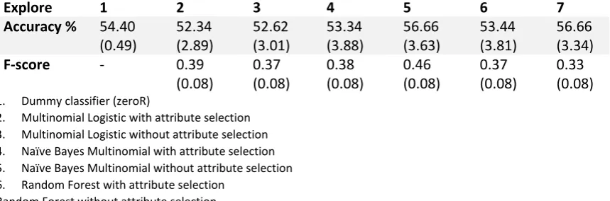
[image:23.595.75.505.312.454.2]

In the final label sessions, some descriptions were not labelled because of the uncertainty. In the previous sections these descriptions were left out of the dataset. However, this influences the representation of the total population. For that reason, another test is performed with a third classification ‘unknown’ for the exploitation and exploration typology. The results are shown in Table 7.

Table 7 Accuracy and F-scores (mean and standard-deviation) classifiers on Explore dataset with a 5-fold cross-validation and 10 repetitions

Random Forest without attribute selection

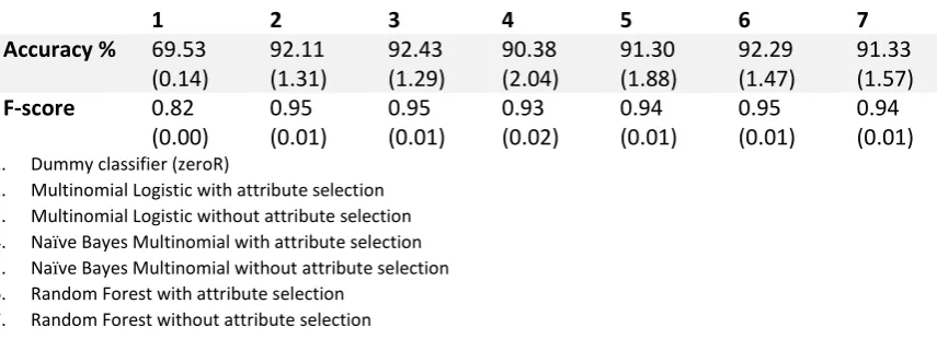
4.1.4 Larger training sample

As a comparison, a prelabelled dataset ‘product, process and software’ was also classified. This unbalanced dataset; product (1458), process (448) and software (191) were less affected by the imbalanced problem as shown in Table 8. The performance on the different classifiers is shown in Table 9.

Table 8 Performance product, process, software

Explore 1 2 3 4 5 6 7

Accuracy % 54.40

(0.49)

52.34 (2.89)

52.62 (3.01)

53.34 (3.88)

56.66 (3.63)

53.44 (3.81)

56.66 (3.34)

F-score - 0.39

(0.08)

0.37 (0.08)

0.38 (0.08)

0.46 (0.08)

0.37 (0.08)

(24)

[image:24.595.76.504.102.257.2]

20

Table 9 Accuracy and F-scores (mean and standard-deviation) classifiers on product, process, software dataset with a 5-fold cross-validation and 10 repetitions

7. Random Forest without attribute selection

4.2 Attribute selection

While the performance of the classifiers on all datasets is low, the attributes that are selected for modelling are comparable with the typology’s theory. The Infogain attribute selection method ranks the attributes based on their information gain. Despite the fact that the exploitation-exploration typology of March is a hard typology to operationalize, the attribute ‘optimization’ has one of the highest ranks in the list of information gain attributes. This attribute is a synonym of ‘refinement’ which is included in March’s exploitation definition. In the push-pull typology the attributes ‘increasing’ and ‘demand’ have a high infogain rank which is in line with the market pull typology. For the underlying dimension ‘architecture’ the attribute ‘application’ has a high Infogain. This could be traced back to ‘another linkage between core concepts’ of the Henderson and Clark typology.

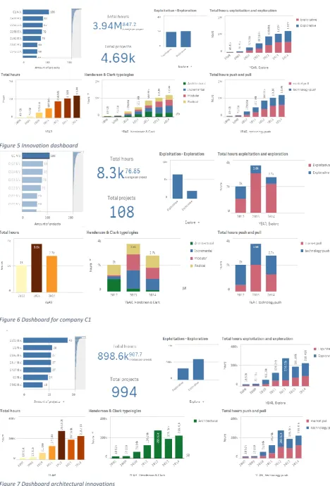
4.3 Interactive dashboard

To show the practical opportunity of this study, an interactive dashboard is built with the predicted labels and the dataset’s additional variables. All projects are shown including the number of project hours and the classified typologies. The dashboard is shown in Figure 5. In the interactive dashboard filters can be submitted. This offers the possibility to produce an overview for just one specific company as shown in Figure 6 or just one typology as shown in Figure 7. An overview of just one year or specific typology can also be submitted. The interactive dashboard is built robust, which means that new predicted data can easily be uploaded in the model.

1 2 3 4 5 6 7

Accuracy % 69.53

(0.14)

92.11 (1.31)

92.43 (1.29)

90.38 (2.04)

91.30 (1.88)

92.29 (1.47)

91.33 (1.57)

F-score 0.82

(0.00)

0.95 (0.01)

0.93 (0.02)

0.94 (0.01)

0.95 (0.01)

(25)

21 Figure 5 Innovation dashboard

[image:25.595.73.542.63.754.2]

Figure 6 Dashboard for company C1

(26)

22

5 Discussion and conclusion

5.1 Discussion

The research goal of this thesis was to investigate the potential of automatic classification of innovation descriptions. To achieve this goal, several sub-questions were added in order to give this research a better structure. The sub-questions will be answered in following sections. The research was started with a literature study in order to answer the following research question:

Q1: Which innovation typologies can be used for measuring innovation portfolios?

As stated by Cocia (2006) there is a lot of inconsistency and overlapping in the innovation’s literature. This is also encountered in this study. There is plenty of literature that describes the importance of balanced innovation portfolios (Cooper, Edgett, & Kleinschmidt, 1999; Macmillian, Hambrick, & Day, 1982) for future possibilities to be recognized (Danneels, 2002), in order to gain a competitive advantage (Brasil & Eggers, 2019). However, there is scarce literature about the consistency between and differences of the innovation typologies.

The OECD distinguishes two types of innovations: product- and process innovation. Besides, Abernathy and Clark (1985) already stated that the type of perspective is the first question for developing a categorization. In addition, Danneels and Kleinschmidt (2001) noticed that firm level is accompanied by familiarity and fit. While customer level is accompanied by risk and adoption. The difference in perspectives was also experienced during the label sessions. For example, a ‘new market’ from a customer’s perspective is the emergence of a totally new market, while from a firm’s perspective this is just a new market for the firm. Therefore, the different perspectives are an important factor for comparing different typologies. Another important factor for comparing the typologies was found in the underlying dimensions. However, not all typologies have clear operationalizations. Some typologies have clear dimensions (Abernathy & Clark, 1985; Booz, Allen, & Hamilton, 1982; Henderson & Clark, 1990), while other typologies are harder to measure (March, 1991; Freeman, 1982; Christensen, 1997). As a result, most typologies can be compressed into six underlying dimensions, namely:

• Technology newness (customer perspective) • Market newness (customer perspective) • Technology newness (firm perspective) • Market newness (firm perspective) • Component newness (product level) • Architectural newness (product level)

In addition, March’s typology ‘exploitation-exploration’ cannot be operationalized into underlying dimensions. The typology ‘market-pull and technology-push’ is a driver of innovation and the typology ‘business-to-business and business-to-consumer’ is used because of possibly good suitability for the current dataset. These dimensions and typologies were used in several label sessions in order to answer the following research question:

Q2: How can the training data be labelled with a high inter-rater-agreement in order to attain a reliable training set?

(27)

23

sessions it became clear that not all dimensions were suitable for this application. The following dimensions and typologies were suitable for current dataset and are used for classification:

• Exploitation – exploration; • Component newness; • Architectural newnesss; • Market pull – technology push;

• Business-to-business or business-to-consumer.

A Cohen’s Kappa of 0.2, 0.34, 0.17, 0.73 and 0.21 was met respectively, which could be interpreted as a poor-, fair- and substantial agreement (Landis & Koch, 1977). This is a small increase compared to the study of Roelofs (2018). Despite the use of underlying dimensions, a code scheme and several label sessions, it was still hard to label due to the high level of abstraction. On the other hand, this implies the potential of automatic classification in order to achieve more standardization. A dataset was created for all labels and used for the machine-learning part of this research. This answers the following research question:

Q3: Which classifiers are best performing?

In the machine-learning part, several problems were found that potentially influence the classifier’s performance. Therefore, these problems will be discussed first. In this project all datasets were imbalanced which led to unreliable trained models, because the classifier tends to label all instances as the majority class. Several methods are used to solve this problem. First, synthetic data for the minority class was created by using SMOTE (Chawla, Bowyer, Hall, & Kegelmeyer, 2002). However, this did not solve the problem. Secondly, cost-sensitive learning was used which assigns a bigger load factor for the minority class (Kao & Poteet, 2007). This also did not balance the dataset. Finally, the datasets were balanced by decreasing the majority class, with the consequence of decreasing the dataset and having less training samples.

The classifiers used on the balanced datasets performed low (highest F-score was 0.65). Subsequently a label ‘unknown’ was added to the instances that were left out during labelling. This resulted in an F-score of 0.46. The training data was increased to a small extent. It did not increase the performance probably due to adding an additional label. To check if a larger training sample would increase the accuracy a new dataset was created. This led to a significant increase with an F-score of 0.95 for a label consisting three classifications. Thereby, the dataset was imbalanced; product (1458), process (448) and software (191), but had barely effect on the performance and confusion matrix. Beside the implication that a larger training set increases the performance, which is in line with the conclusion of Roelofs (2018), it also decreases the imbalance problem.

Another important conclusion is that the attributes that were selected had similarity with the innovation’s theory. For example, for the label ‘exploitation’ of March (1991) the attribute ‘optimization’ had one of the best infogain scores and is a synonym for the word ‘refinement’ which is included in March’s definition. This implies that the classifier can find theory-based attributes by itself. On the other hand, it might be possible to increase the accuracy of the classifier. However, overfitting is lurking because the classifier could use non-informative attributes which are only meaningful for the relevant data, with the result that it is not applicable on other data.

(28)

24

Q4: How can the predicted data be used for practical contribution?

Even though the accuracy for the models was low, the practical potential of this automation is shown with the interactive dashboard. This tool can be used for measuring the consultancy firm’s KPI’s, an innovation scan could also easily be performed for all their clients separately. Thereby, the dashboard is robust so new results can easily be added to the current tool and a business list of active products and new R&D projects can easily be updated. The resources spend on each project are well-arranged by using the project hours. This tool can be used to determine the current product portfolio (Macmillian, Hambrick, & Day, 1982) and recognizing future opportunities (Danneels, 2002).

5.1.1 Limitations

Besides the positive contribution of this research, several limitations appeared. To start with, the data that was used is not totally representative for the market. The data is from one consultancy firm and companies may not provide all their innovation projects to this firm, so their innovation portfolio might be not totally represented in this dataset. In addition, descriptions are used for grant application what makes it somewhat unreliable. However, the dataset contains many different industries, companies and applications. The descriptions were also different in some cases. Some descriptions are different in document length, informative about company’s background or have less focus on technical aspects of the project. There are also cases were different small projects are described in just one application what makes it harder to classify, especially for the ‘architectural’ and ‘component’ dimensions.

A second limitation is the manual classification of the training data. The underlying dimensions and typologies still have a level of abstraction which makes it difficult the achieve a high level of agreement between the coders. This is also shown in the final sample, because many descriptions are labelled as ‘unknown’.

Finally, there are some limitations in the machine-learning performance. In this project, only Weka was used for training the samples. In the research of Roelofs (2018) the project was implemented in Python. However, the same classifier algorithms were used, some difference in programming sequences possibly influenced the results.

5.2 Conclusion

This research was done in order to answer the research question: ‘How can innovation descriptions automatically be classified using a machine learning approach, and which conclusions can be drawn of the sample’s portfolio trends?’. Machine-learning based classification of innovation descriptions is a promising method for practical and theoretical applications. However, as discussed in previous section, this research has come across several difficulties which negatively influenced the reliability of the classification. This research has delivered a foundation for further research, whereas underlying dimensions were clarified and the application of these dimensions on the data was performed. It is unfounded to make statements of the innovation portfolio trends because of the low performance of the classifiers. Instead, this research has delivered a working and robust tool where trends can be visualized easily.

5.2.1 Further research

(29)

25

dataset could be used. The dataset used in this research including a wide range of companies in different industries with the advantage of the generalizability of the model, but also had a negative influence on the required training data. A more specific dataset could possibly achieve a higher accuracy. In addition, a prelabelled dataset could increase the accuracy of the model as well as the lead time of the research. A pre-labelled dataset will solve the manual labelling problem as well.

Secondly, the underlying dimensions and typologies could be used for further research on economics of innovation. Using the underlying dimensions will make academic research, as well as innovation portfolios, more consistent and thus comparable to each other. During the label session the data set also seemed appropriate for classification of marketing strategy purposes like the Ansoff matrix.

In the future this dataset could also be expanded with the previous collected data. Also, other variables could be added like financial performance indicators and industry or economic figures. The individual result of the grant application could also be an interesting input variable, because the eligibility of the grant application could be tested by the model.

(30)

26

Appendix A: Code scheme

Innovation process

1. Organizational learning (innovation process) • Firm level perspective

Exploitation 1 2 3 4 5 6 Exploration

The innovation requires firm’s existing knowledge.

The innovation requires new knowledge

Technological knowledge facilitates a process of exploitation by refining and extending existing competencies and technologies, science facilitates a process of exploration by experimenting with new competencies and technologies (March, 1991).

Product

Example components/architecture: A room fan’s major components include blade, the motor, the blade guard, control systems and the mechanical housing.

The overall architecture of the products lays out how the components will work together. A fan’s architecture and its components create a system for moving air in a room (Henderson & Clark, 1990).

2. Newness components (product) • Product level

• Technological discontinuity

Low 1 2 3 4 5 6 High

The product’s components are reinforced / unchanged

The product’s components are overturned / changed

dramatically (e.g. analog to digital tv)

3. Newness architecture (product) • Product level

• Technological discontinuity

Low 1 2 3 4 5 6 High

The linkages between the core concepts and components are unchanged

(31)

27

Incentive / market

4. Market pull – technology push (incentive innovation process) • Market / Micro level (customer needs)

• Marketing discontinuity

• As incentive for the innovation

5. B2b – b2c

Market pull 1 2 3 4 5 6 Technology push

Innovation based on market demand

Innovation based on own incentive

Business to consumer 1 2 3 4 5 6 Business to business

Selling innovation directly to consumer

(32)

28

Appendix B: Pre-processing

[image:32.595.71.536.145.362.2]

The settings of the string to word vector are shown in Table 10.

Table 10 String-to-word-vector settings

Weka Filter String-to-word-vector

IDFTransform True

TFTransform True

AttributeIndices First-last

Debug False

DonotCheckCapabilities False

DoNotOperateOnPerClassBasis False

InvertSelection False

LowerCaseToken True

MinTermFreq 1

NormalizeDocLenght No normalization

OutputWordCounts True

PeriodPruning -1.0

SaveDictionaryInBinaryForm False

Stemmer SnowballStemmer S – Porter

StopWordsHandler Words from file

Machine learning classification tool for innovation projects