http://go.warwick.ac.uk/lib-publications
Original citation:Mao, Lei and Tserlukevich, Yuri (2013) Repurchasing debt. Working Paper. (Unpublished)
Permanent WRAP url:
http://wrap.warwick.ac.uk/55509
Copyright and reuse:
The Warwick Research Archive Portal (WRAP) makes this work by researchers of the University of Warwick available open access under the following conditions. Copyright © and all moral rights to the version of the paper presented here belong to the individual author(s) and/or other copyright owners. To the extent reasonable and practicable the material made available in WRAP has been checked for eligibility before being made available.
Copies of full items can be used for personal research or study, educational, or not-for-profit purposes without prior permission or charge. Provided that the authors, title and full bibliographic details are credited, a hyperlink and/or URL is given for the original metadata page and the content is not changed in any way.
A note on versions:
The version presented here is a working paper or pre-print that may be later published elsewhere. If a published version is known of, the above WRAP url will contain details on finding it.
Repurchasing Debt
Lei MAO and Yuri TSERLUKEVICH
June 2013
Abstract
In this paper we build a theoretical model of corporate debt repurchases. First, we
…nd that the …rm that buys back its own debt from a creditor must pay a premium
over the price at which the same creditor is willing to trade with third parties. This is
because the repurchase by a …rm leads to a dollar-for-dollar reduction in the amount of
cash or assets available to pay the remaining debt. Second, the repurchase price is lower
when there are multiple bondholders because of cross-creditor externalities. Therefore,
we challenge the view that restructuring more dispersed debt is always more costly to
implement. Third, when bankruptcy costs are signi…cant, there is a range of prices
below face value at which debt can be repurchased. Fourth, we show that repurchases
contribute to ‡exibility in …rms’capital structure and increase ex-ante …rm value, but
have limited power to mitigate debt overhang.
JEL codes: G32 Keywords: Savings, Debt Repurchase, Debt Overhang
1. Introduction
The low price of corporate debt in the secondary securities market and recent tax
in-centives arising from the post-crisis American Tax Recovery and Reinvestment Act of 2009
presented an opportunity to many …rms to restructure or reduce outstanding debt on more
favorable terms. By repurchasing their debt with cash or assets, companies were able to
reduce their existing indebtedness (which carries no tax advantage net of cash) at less than
the original face value, reduce their interest costs, and remove restrictive covenants. In
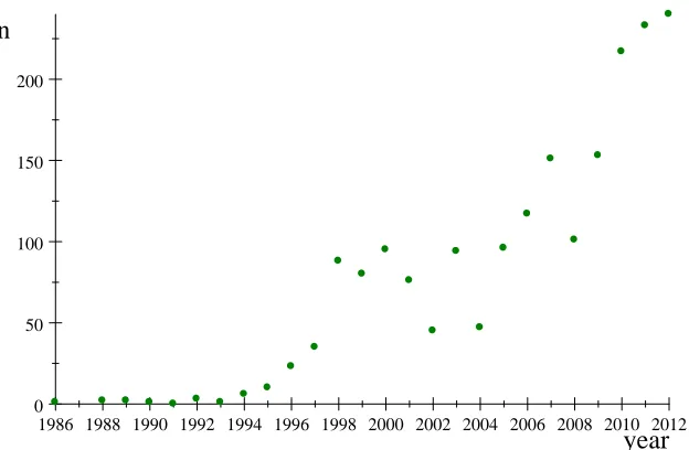
2010, for example, companies initiated 190 cash repurchases of publicly traded bonds, with
an aggregate amount of $36.3 billion, compared to just 49 transactions during the period
1986-1996 (see Figure1).1 Despite the increasing number of debt repurchases, the academic
literature on this topic is virtually nonexistent. In this paper, we provide a formal theoretical
framework for corporate debt buybacks, with the goal of understanding when a repurchase
is optimal, and what the implications it has for shareholders and creditors. The framework
lends itself to a number of applications and empirical predictions.
First, we show that creditors should not sell risky debt back to the company at the
market price–i.e., the price at which they would be willing to trade with third parties. We
provide an example of a …rm with a sole lender or a group of coordinated lenders, under
Modigliani-Miller conditions. In this frictionless setting, the minimum price at which the
lender agrees to sell the marginal unit of risky debt back to the …rm is equal to the face value
of the debt, above the market value. All additional bonds are also repurchased at the face
value. Note, however, that it is impossible to buy back all debt at the face value, since if
there were enough cash to do this, the debt would not be risky. The basic idea is that using
cash or any safe asset for repurchase adversely a¤ects the value of the remaining debt claims
and does not reduce the probability of bankruptcy since the …rm’s liabilities and assets are
1These estimates are conservative because many repurchases are not recorded in the FISD database. They
reduced by the same amount. In essence, the debt is secured by cash and assets inside the
…rm, so that repurchasing the debt amounts to paying the lender with his own money.
Second, debt that is held by many shareholders can be repurchased at a signi…cantly lower
price. Bonds can be repurchased on the open market or using a tender o¤er at prices close
to the market price, as long as there are small investors willing to sell their entire stake.
The important di¤erence from the frictionless case is that the sellers do not internalize a
decline in the value of the remaining debt because it is held by other investors. We show
that the equilibrium outcome in this case depends on the price o¤ered in the repurchase.
The repurchase is guaranteed to be successful for any o¤er price above the market price,
and may even be successful for prices below the market price if investors are optimistic
about the repurchase completion. Intuitively, there is a strong incentive to participate in the
repurchase because the price is expected to decrease. Those investors that do not tender or
exchange their bonds are exposed to increased risk and lower value.2
Third, we discuss bankruptcy costs, tax, and transaction costs in the context of our
model, and show that (1) costly bankruptcy encourages repurchases; and (2) taxation and
transaction costs discourage repurchases. Intuitively, …xed and proportional bankruptcy
costs decrease recovered value to a lender following …rm default and therefore encourage
bondholders to make concessions. The model gives a range of prices at which a repurchase is
possible. Within this range, the negotiated price depends on the relative bargaining power
of shareholders and bondholders. Expected bankruptcy costs in repurchases are reduced
in two distinct ways. Cash or assets transferred to creditors before bankruptcy reduce the
proportional bankruptcy costs. Additionally, the repurchase at a price below the face value
reduces the probability of bankruptcy. Taxation is shown to a¤ect the repurchase incentive
primarily through cancellation of indebtedness (COD) tax, which results in an additional
cost proportional to the size of the repurchase discount.
Fourth, we argue that, from the ex-ante perspective, the ability to repurchase debt is
2There are legal restrictions applicable to the tender o¤er repurchases of publicly traded debt, that
bene…cial to the …rm. Repurchasing at prices below the face value— e.g., through the tender
o¤er— increases …rm value and the …rm’s debt capacity. Although bondholders may be
exploited ex-post, the overall e¤ect on …rm value is positive because shareholders gain more
than bondholders lose. We discuss features of creditor structure and debt contract design
that decrease the …rm’s ability to repurchase debt because they will also decrease …rm value.
For example, it is easier to repurchase publicly traded debt because there are small investors
who can sell their entire stake. At the same time, we …nd that convertible debt is harder to
repurchase because of the additional regulatory requirements. Contrary to casual intuition,
a call option has little e¤ect on the value of the repurchase option since the former is in the
money when the debt value is high, and the latter when the debt value is low.
Although a repurchase reduces …rm indebtedness, we show that in most cases it cannot
mitigate agency con‡icts originating from debt, such as the underinvestment problem. At
the root of the problem is the condition that, unless the repurchase price is lower than the
face value, the bankruptcy risk and debt overhang will not be a¤ected by buying back debt.
We further show that it may be impossible to negotiate a lower repurchase price because
bondholders require a premium in anticipation of the investment. Finally, we show that a
…rm with severe …nancial constraints will be better o¤ if it allocates cash directly to the
investment instead of …rst undertaking a debt repurchase.
The analysis here also provides insights on debt repurchase timing. It is clear that
buying back debt is costly and at least partially irreversible. Because the expected gain
from a repurchase increases with the risk of default, managers have an incentive to postpone
the repurchase until a date closer to debt maturity. Therefore, the option to buy back debt
must be kept “alive”by increasing cash reserves instead of immediately reducing debt. It is
therefore important, going forward, to recognize that shareholders may intentionally engage
in simultaneous borrowing and saving to increase the value of the repurchase option.
This paper is related to the literature on debt restructuring and debt exchanges. Since
Dornbusch (1988), and Gertner and Scharfstein (1991), who focused on implications of the
sovereign and corporate debt exchanges prevalent in the 1980s, ours is the …rst formal study
to address the current phenomenon of corporate debt repurchases.3 Gertner and Scharfstein
(1991) show, in particular, that o¤ering new senior securities (cash paid to debtholders
is one example of such a security) in exchange for distressed junior debt is bene…cial to
shareholders. However, Gertner and Scharfstein (1991) do not discuss the price, optimal
timing, and the determinants of debt repurchases, which are the focus of our paper. Froot
(1989), Bulow and Rogo¤ (1991), Bulow, Rogo¤, and Dornbusch (1988), and others study
open-market sovereign debt repurchases in the presence of the debt overhang problem. The
major di¤erence between corporate and sovereign debt buybacks is that, in the latter, cash
and assets cannot be meaningfully pledged (see Bulow, 1992, for details).
Our work is also related to the strategic debt service literature (Mella-Barral and
Per-raudin, 1997, Hart and Moore, 1998). Firms facing …nancial distress can act strategically
and force concessions from debtholders. However, whereas strategic debt service deals with
bargaining after default, when cash e¤ectively already belongs to creditors, we discuss
repur-chases by a solvent …rm. For this reason, some of the predictions in our model are contrary
to those in the debt renegotiation literature. For example, we show that the dispersion of
debtholders that is commonly seen as an impediment to renegotiations actually helps to
reduce leverage and the probability of bankruptcy in debt repurchases.
Our results have connections to the literature that investigates investment, debt, and
the propensity to save in …nancially constrained …rms. For example, Acharya, Almeida, and
Campello (2007) describe the intuitive trade-o¤ between saving cash and repurchasing risky
debt when investment opportunities are positively correlated with cash ‡ows and debt can
be purchased at the market price. We extend their results by laying out the conditions
that determine the repurchase price. Finally, our study is related to the growing literature
3In related empirical studies that focus on debt exchanges and repurchases, the propensity for debt
that examines the role of cash holdings within dynamic models and sheds light on the large
observed cash accumulation.4 We show that saving cash can be bene…cial when the …rm
anticipates future debt repurchases.
2. Institutional Background
There are three main mechanisms for buying back corporate debt: open-market
repur-chase, tender o¤er, and privately negotiated repurchase.5 An open-market repurchase, which
includes repurchases in private markets by institutional buyers, is executed over a period of
time and allows for potentially di¤erent prices for each bond sold back to the …rm. A tender
o¤er is typically conducted by o¤ering a single price to all bondholders. Repurchases are
conducted using cash savings, proceeds from the sale of assets or proceeds from senior
secu-rity issuance collateralized by these assets (Gertner and Sharfstein, 1991). In this paper, we
do not discuss debt-for-equity exchanges, which have di¤erent implications.
An open market repurchase is an easy way for an issuer to buy back relatively small
amounts of debt. Other than complying with the anti-fraud provisions of the federal
se-curity laws, these transactions are not normally subject to review by the U.S. Securities
and Exchange Commission (SEC).6 However, it is di¢ cult to repurchase large amounts in a
limited time on the open market. Also, this mechanism does not permit the issuer to amend
the covenants of the bonds because the issuer or the a¢ liates are not entitled to vote for the
purpose of giving consents under the indenture.
Tender o¤ers can include a …xed premium over the current trading price and allow the
repurchase of larger amounts. Importantly, tender o¤ers may include additional incentives
for bond investors, which all but guarantee a successful repurchase. To motivate the holders
4For example, Morellec and Nikolov (2009) and Hugonnier, Malamud, and Morellec (2011) link cash
holdings to investment, competition, and a desire for liquidity. In Riddick and Whited (2009), saving policy trades o¤ tax penalties and the reduction in expected future …nancing costs.
5Debt repurchases may also be conducted as auctions. For example, Hovnanian Enterprises Inc. used a
modi…ed Dutch auction with base bid prices ranging from $480 to $750 per $1,000 of the face value. The company eventually paid $223 million to buy back $578 million of debt in February and April of 2009.
6However, issuers may face greater regulation by the SEC if they proceed with very large repurchases
of bonds to tender without o¤ering a large premium and to avoid the need to comply with
all of the existing contractual requirements, companies also solicit “exit consents”with their
o¤er, in which case the holders of the securities are asked to consent to amendments to the
security as a condition of their acceptance of the o¤er (Kaplan and Truesdell, 2008). If the
consent solicitation is successful, any holders who refuse to accept the o¤er would continue
to hold their old securities, which are stripped of protective covenants and made e¤ectively
junior to the new security.
An additional advantage of conducting a tender o¤er with “exit consents” is the ability
to remove existing covenants that restrict the borrower’s future actions (Mann and Powers,
2007). Having removed these covenants, the company may gain more ‡exibility in investment
and …nancing decisions. For example, a …rm may be able to increase capital expenditures,
make an acquisition, increase dividends, liquidate assets, transfer money to subsidiaries,
change the …nancial reporting procedure, alter collateral, consolidate assets, merge with
another company, change lines of business, or modify its bylaws (Roberts and Su…, 2009,
and King and Mauer, 2000).
However, there are two serious di¢ culties that companies must overcome. First, tender
o¤ers for publicly traded debt require compliance with the Trust Indenture Act of 1939,
section 316(b), which prohibits debtholders from changing the principal of debt without the
debtholders’unanimous consent. It is designed, in particular, to prevent the company from
exploiting minority bondholders. Managers can (and do) avoid this restriction by buying
back a portion of debt on the open market or by combining cash repurchases with exchanges
for other securities (see, e.g., Brudney, 1992, Gertner and Scharfstein, 1991, and Shuster,
2007).7 They can also avoid having their repurchase classi…ed as a tender o¤er by soliciting a
limited number of holders, repurchasing over a fairly long period of time, and/or purchasing
on di¤erent terms from each holder.
7Shuster (2007) gives examples of the provisions, which were originally designed to remove small
Second, whenever debt is repurchased below its face value, the …rm is subject to a tax
on the COD income. Unless an exception applies, such as insolvency or bankruptcy at the
time of the repurchase, shareholders must recognize the COD income upon satisfaction of its
indebtedness for less than the amount due under the obligation. The COD income is usually
the di¤erence between the amount due under contract and the amount paid.8 Firms facing
COD may …nd that the additional tax partially o¤sets the bene…ts of buying back debt at a
low price. However, the recently enacted American Recovery and Reinvestment Act allows
deferring the COD tax costs for up to 11 years, e¤ectively making debt repurchases more
attractive.9
3. Model of Debt Repurchase
In this section, we lay out the basic single-date model in the frictionless case with a
single bondholder. Later we relax some of the assumptions of this framework and analyze
how di¤erent …nancing frictions a¤ect debt repurchases.
3.1. The Frictionless Case
Suppose that the …rm has cash C, or a liquid riskless asset of an equivalent value, or
proceeds from a senior security collateralized by this asset. The existing assets of the …rm
generate a cash ‡ow x, distributed according to the cumulative distribution function F(x)
on the non-negative support [X; X]. If cash ‡ows can be negative, X < 0, we rede…ne
C0 =C+ min(X); if the …rm can spend only part of available cash on debt repurchase, then
C contains only this part. We assume that all of the …rm’s debt D (including accumulated
interest at rate r) matures shortly after realization of x. Since the problem is trivial in the
8This di¤erence and the associated COD tax can be non-trivial. For example, Harrah’s paid about 48
cents on the dollar to repurchase $788 million of debt in the second quarter of 2009. If not for the ARR tax deferral, Harrah’s would face an immediate COD tax levied on the discount of about $400 million.
9The act does not alter how COD income arises, but rather a¤ects when the debtor pays tax on the
case of riskless debt, we require that the …rm defaults in at least some states of the world,
i.e.,
C+X < D C+X: (1)
If the …rm becomes bankrupt, the priority rule is observed and debtholders have …rst
claim on the …rm’s assets. In the frictionless model, we assume that there are no costs
associated with bankruptcy. Additionally, since our objective is to determine the impact of
a …rm’s …nancial position on the incentive to increase or decrease leverage, we assume that
the …rm “inherits” debt and postpone the discussion of optimal leverage until Section 5.
Lenders assume equal seniority; however, future debt issues are restricted to subordinate
claims only and do not a¤ect the recovered amount of the senior lender in the event of
default.
We …rst consider debt held by a sole lender, such as a private investor, or alternatively
several large lenders, who collude when negotiating the sale price of debt. We assume that
the …rm is restricted from paying dividends or conducting share repurchases because such a
distribution of cash would result in the value transfer from the lenders to the shareholders.
Provisions limiting distributions a¤ecting debt repayments are commonly included in debt
covenants (Smith and Warner, 1979). Obviously, if unlimited dividends or share repurchases
are allowed before the principle amount of debt comes due, shareholders’…rst-best strategy
entails selling all assets to maximize the payout. Shareholder-debtholder con‡icts are trivially
resolved in this case (see, e.g., Jensen and Meckling, 1976). Finally there are other uses for
…rm’s cash, which we do not allow in a simple model, such as investment considered in the
later sections of this paper, compensation to employees, or perks to the management.
The objective of the manager is to maximize the value of equity with respect to …nancing
decisions. In particular, the manager considers two alternative strategies: saving amount
C, or using cash to repurchase an amount of debt D from the lenders. Note that the
average repurchase price is PR = C= D; for example PR = 1 means that repurchase is
is, the repurchase does not generate any synergies that can increase the value of the assets
and therefore lead to the bondholder hold-out problem (similar to, e.g., Shleifer and Vishny,
1986).
We derive the repurchase price restrictions from the participation conditions for equity
and debt holders. De…ne the equity value as S0
S0 =
Z X
D C
(x+C D)dF(x): (2)
De…ne the equity value if the …rm buys back Dof outstanding debt using all available cash
C asSR
SR =
Z X
D D
[x D+ D]dF(x): (3)
Similarly, de…ne the market values of debt as, respectively, d0 and dR
d0 =
Z D C
X
(x+C)dF(x) +D
Z X
D C
dF(x); (4)
dR=
Z D D
X
xdF(x) + (D D) Z X
D D
dF(x): (5)
Note that, because of assumption (1), the initial price of debt is below face value, P0 =
d0=D <1. The following proposition links equity and debt values to the price of the
repur-chase.
Proposition 1 Under the assumptions of the frictionless case, the following statements are
equivalent
PR<1;
SR> S0;
dR+C < d0: (6)
The proposition says that, if the repurchase price is lower than the face value, shareholders
are better o¤ after the repurchase and the bondholders are worse o¤. It follows that the
face value is the only price at which both sides agree to buy and sell debt. Note that the
repurchase price is unique because in the frictionless case debt repurchase does not change
the total value of the …rm. However, we show in the next section that there is a range
of acceptable prices in case when the …rm’s assets are subject to bankruptcy costs. The
prospect of reducing bankruptcy costs makes room for negotiations between shareholders
and bondholders.
3.2. Bankruptcy Costs
Here we assume that in the event of default lenders take over the …rm and implement
…rst-best policies, subject to a fraction of the …rm’s assets being lost during the transfer.
Firm entering bankruptcy results in …xed cost, B, and proportional cost , which is known
both to shareholders and to creditors. Unlike in, e.g., Leland (1994), we recognize that safe
assets may be di¤erent from risky assets and assume that cash or liquid assets are subject
to cost 1 2(0;1), and other assets are subject to cost 2 2(0;1). Although not crucial for our argument, it may be reasonable to conjecture 1 < 2, meaning that safe/liquid assets are easier to transfer to new owners. Parameter 1 can also be interpreted as the agency
cost, such as the manager’s ability to “burn” cash before bankruptcy.
The expected bankruptcy costs are therefore
BC0 =
Z D C
X
( 2x+ 1C+B)dF(x): (7)
The following proposition gives the upper and lower bounds for the repurchase price
and shows that the repurchase price is lower in the case with bankruptcy costs than in the
frictionless case.
B >0; 1 >0, 2 >0, and that, except for bankruptcy costs, assumptions from the friction-less case hold. Then
PR2[PRmin;1];
where the lower bound on the repurchase price, Pmin
R <1, is the unique solution to equation
(26) in the Appendix.
Intuitively, if shareholders have all bargaining power in splitting the surplus from the
bankruptcy costs reduction, the lowest price, Pmin
R , is obtained. If, instead, bondholders
have all bargaining power, then debt is repurchased at the face value, as in the frictionless
case.
Because the bankruptcy costs decrease, …rm value increases after the repurchase. From
Proposition 2 and expression (7), …rm value increases by
(BC) = C 1
Z D C
X
dF(x) +
Z D C
D D
(B + 2x)dF(x): (8)
Bankruptcy costs decrease, intuitively, for two reasons. First, during the repurchase, cash
(or safe asset)C is transferred directly to bondholders in exchange for lower debt. It matters
because, if the …rm subsequently defaults or becomes bankrupt, this cash or asset, which
are inside the …rm, would be subject to the proportional cost 1.10 Therefore, expected
bankruptcy costs are reduced even if the probability of bankruptcy is …xed, as captured in
the …rst term in (8).
The second e¤ect arises because repurchases generally lead to a lower probability of
bankruptcy. Because of the reduction in proportional bankruptcy costs, a lower repurchase
price can be negotiated, resulting in an additional bene…t in the form of lower bankruptcy
risk (the second term in (8)).
Overall, we predict that the average debt repurchase price is lower when expected
bank-10Cash is subject to bankruptcy costs, even if the …rm can eventually restructure and exit the bankruptcy.
ruptcy costs are higher. Additionally, keeping bankruptcy costs parameters …xed, the
repur-chase price increases with relative bargaining power of bondholders.
3.3. Multiple Bondholders
We model a single-date same-seniority (“pari passu”) debt repurchase from a group of
identical bondholders, each holding the same small share of debt. When the …rm has
out-standing debt of di¤erent seniorities, the argument extends to the most senior debt.
Some-times, in addition to the senior debt, the companies also attempt to buy back their junior
debt. For example, the 2009 Royal Bank of Scotland tender debt repurchase o¤er included
subordinated notes. However, understanding repurchase o¤ers for junior debt is complicated
because they lead to an additional con‡ict between the di¤erentclasses of the bondholders.
Additionally, we assume in this section that revolving credit facilities and other
high-priority obligations are repaid before the price for senior debt can be negotiated, debtholders
are fully rational and attentive, and there are no bankruptcy costs or other …nancing frictions.
Consider …rst a tender o¤er, when a …xed price is o¤ered to everyone who sells their
bonds. If all bondholders tender simultaneously, they are served sequentially in random
order until the full amount allocated for this purpose is spent. There is usually no minimum
subscription requirement for the o¤er. It is intuitive that the tender o¤er equilibrium is
contingent on how the o¤er price, P, compares to the pre- and post-repurchase prices.
For example, if the tender o¤er price is high, the bondholders will participate because the
expected post-repurchase price,PR, is going to be lower. If the tender o¤er price is low, the
bondholders will all abstain because the debt price without the repurchase,P0, is higher. As
the …rst step in formalizing this intuition, we de…ne a “…xed-point” price, PF, at which the
post-repurchase price remains exactly the same as the o¤er price.
Lemma 1 Suppose debt is repurchased through the tender o¤er from multiple bondholders:
(i) there is a unique …xed-point tender o¤er price PF, such that PF P =PR,
(ii) PF < P0.
The Lemma de…nes the …xed-point price and states that it is strictly lower than the
pre-repurchase price. According to the Lemma, repurchasing debt at any price above the
…xed-point price (including the pre-repurchase price) will decrease the value of the bonds for
the remaining bondholders.
Next, we discuss possible equilibria. First, we consider the case when the tender o¤er
price is high, above the pre-repurchase and the …xed-point price, P P0 > PF. From
Lemma 1, the bondholders who do not tender receive a strictly smaller post-repurchase
price, PR < P0. Therefore, there is a unique equilibrium in this case: the …rm o¤ers a price
equal to or just above P0, all bondholders tender, and a fractionC=(P D)of them are served
randomly until all cashC is spent.11
Second, consider a tender o¤er price between the pre-repurchase price and the …xed-point
price,P0 > P > PF. The equilibrium in this region depends on the beliefs about the number
of bondholders participating in the repurchase.
Proposition 3 Suppose the tender o¤er price P 2 (PF; P0). If every bondholder has a
uniform belief j about the fraction of bondholders who will participate in the o¤er, then:
1. for j j , all bondholders tender, and the tender o¤er is successful.
2. for j < j , all bondholders abstain from the tender o¤er, and the o¤er fails.
The threshold belief j 2 (0; C=(P D)) is given as a unique solution to the equation (32) in
the Appendix.
The proposition gives the threshold belief regarding the fraction of tendering bondholders,
which can trigger the “bank run” (Diamond and Dybvig, 1983). For example, if the belief
about the success of the o¤er is highly optimistic, i.e., j !1, then it implies PR < P, and
the o¤er is successful as nontendering bondholders are expected to be worse o¤. In contrast,
11A parallel result to this case can be found in Dhillon, Noe, and Ramirez (2001), who show that
j !0 implies that PR > P, and the o¤er fails. Following Diamond and Dybvig (1983), we
treat belief j as exogenous.
Finally, any tender o¤er price, which is equal to or below the …xed-point price, trivially
leads to the repurchase failure. By the de…nition of the …xed point, for any P PF and
any belief j, the post-repurchase price is expected to increase, PR P, and therefore every
bondholder will abstain from tendering.
Intuition for the open-market debt repurchases is similar to the tender o¤er case. An
important di¤erence, however, is that bondholders may receive di¤erent prices for their
holdings, depending on the relative timing of the sale. As we have argued, the price for
the remaining debt will decrease with each repurchase at the price above the …xed point,
including the market price. Therefore, bondholders have a strong incentive to participate,
and those who sell …rst will receive the best deal. At …rst, this may appear counterintuitive
because a debt reduction would seem to make the remaining debt safer. Instead, a repurchase
consumes cash inside the …rm, making the remaining debt riskier. We do not formally de…ne
the equilibrium for the case of open market repurchases as it requires modeling heterogeneity
among bondholders and building a sequential game for the stages of the repurchase.
There are two other important points that we would like to bring to light in conjunction
with the case of multiple bondholders. First, we have assumed throughout that each investor
holds an identical small fraction of debt and sells it entirely to the …rm. Such continuum
of homogeneous investors is a su¢ cient condition for our results, but not a necessary one.
For example, when the creditor composition involves both large and small investors, debt
will …rst be repurchased from the small investors. These investors can sell their entire debt
holding in response to the o¤er and do not need to internalize the consequences of the
repurchase on the outstanding debt.
Second, the news of the incoming tender o¤er, including information on the size of the
o¤er and its outcome, may alter the market prices for both debt and equity. Speci…cally,
of debt lower than the initial price. Recall that the initial price,P0 is de…ned as the expected
payo¤ to bondholders if the repurchase is not anticipated, or if it is not expected to be
successful. The Appendix provides the expression for the market price with the adjustment
for the repurchase, which may be di¤erent from the initial priceP0. It is important, however,
that the equilibrium does not depend on the true market price. It depends only on the
relation between the tender o¤er price, the price if the repurchase fails, P0, and the
…xed-point price PF.
The main insight from our study of the dispersed creditors case— debt held by multiple
bondholders can be repurchased at a lower cost— contrasts sharply with the predictions
of the literature on debt renegotiation and strategic debt service (e.g., Hart and Moore,
1998; Mella-Barral and Perraudin, 1997). Like in this literature, shareholders in our model
are able to force concessions from debtholders. However, the strategic debt service deals
with bargaining after default, when cash e¤ectively already belongs to creditors and the
negotiation is purely targeted to reduce bankruptcy costs. For this reason, small bondholders
in their models, who can either abstain from negotiations or demand a premium, free-riding
on large bondholders, make debt renegotiation impractical. The distinction must be made,
because existing literature on the topic often draws conclusions on the basis of the debt
renegotiation theory. For example, Mann and Powers (2007) argue that tender o¤ers are
easier to complete in …rms with more concentrated debt ownership.
3.4. Tax and Transaction Costs
As we have argued, the discounted repurchases are bene…cial to the shareholders; however
these bene…ts are likely to be reduced by transaction costs and tax. First, we discuss the
tax implications of repurchasing debt versus saving cash. As is standard in the literature
(see, e.g., Auerbach, 2001), we track the after-tax payo¤ to shareholders under the two
alternatives. If the …rm saves C for one period, the after-tax dividend to shareholders is
assuming that tax Tc is levied on corporate income and cash distributions are subject to
further tax at the rate Td. Alternatively, if the …rm repurchases a portion of its debt, D,
the after-tax dividend
Payo¤Rep = D(1 +r(1 Tc)) (1 Td) (10)
TCODmax( D C;0)(1 Td);
where the second term is an additional tax on the COD income if debt is repurchased at a
discount. From (9) and (10), we compute the debt repurchase tax advantage over saving as
AdvRep = ( D C) (1 +r) ( D C)rTC (11)
TCODmax( D C;0):
The direct bene…t of repurchasing debt at a discount (…rst term) is reduced by a higher
corporate tax due to the lower debt-net-of-cash (second term) and also a higher COD tax
(third term). We compare this expression to our base model and conclude that corporate
and COD tax reduce the ex-post bene…ts from the repurchase.
Transaction costs, trivially, can also reduce the repurchase incentives, and therefore must
be considered against bene…ts of the repurchase. Firms incur signi…cant direct and indirect
costs when conducting debt repurchases, including premia paid in the tender o¤ers and open
market purchases. Costs associated with amending the contracts as well as attorneys’fees can
also be signi…cant (see, e.g., Roberts and Su…, 2009). Finally, large indirect fees commonly
appear, which take the form of time and e¤ort spent by both borrowers and lenders on
understanding the implications of the transaction, and obtaining approval or waivers in case
of syndicated loans.
Overall, we …nd that bankruptcy costs and dispersed debt ownership, two assumptions
that are common to U.S. …rms, result in a lower repurchase price. With moderate transaction
immediate repurchase, we show in the next section that treating the repurchase as an option
and delaying its exercise results in higher expected pro…ts.
4. Multi-Period Extension
We previously adopted the assumption that debt must be repurchased on a single date.
This section extends the previous analysis by studying the intertemporal debt/cash policy in
a two-period model. Such model allows us to understand what determines the optimal timing
of debt repurchase and in particular the shareholder’s incentives to delay the repurchase.
4.1. Frictionless case
Assume there are three dates, t = 0, 1, 2, and values are denominated in date t = 0
dollars. The …rm’s total pro…t at the end datet= 2 is equal to the sum of the independently
distributed pro…ts from the …rst and the second period, x1 +x2, where x1;2 2 [X; X]. At
t= 1, the information aboutx1 becomes available, and at datet = 2, the information about
x2 becomes available.
Equity maximizes the expected payo¤ with respect to saving/debt reduction decisions.
Since the model now extends beyond a single period, we need to adjust the subscript notation
accordingly. Assume that the initial face value of debt is D0 and that it can be reduced to
D1 (before pro…t x1 is revealed). At the next date, D1 can be further reduced toD2 (before
x2 is revealed). Similarly, we denote the cash changes due to the …rst and second repurchases
as C0 C1 and C1 C2. Observing from Proposition 1 that at t = 2 shareholders bene…ts
from buying the maximum amount, we set C2 = 0.
In absence of intermediate dividends, the objective function of the shareholders is the
expected value of the payo¤ at the last datet = 2
max
(C1)
V0 =
Z X
X
"Z X
D2(C1) x1
(x1+x2 D2(C1))dF(x2)
#
dF(x1); (12)
abuse of terms, the derivative of this function,@V0=@C1, can be interpreted as “propensity to
save”or “propensity not to reduce debt,”used in prior literature. To maximize equity value,
the manager minimizes the …nal-period debt value with respect to the repurchase policy.
Lemma 2 In the frictionless case timing of the repurchase is irrelevant.
It is straightforward to see from (12) why in the absence of frictions equity value is
independent of repurchase timing. In this case, the price equals to the face value, regardless
of the time of the repurchase, and cash simply cancels an equal amount of debt,D2 =D0 C0.
It is important to recognize that the irrelevancy result exists in the frictionless case because
the …rm never “regrets” undertaking repurchases at the …rst date. Below we show that the
timing matters outside of frictionless case.
4.2. The option to delay debt repurchases
Suppose the …rm can repurchase on the open market at the current market price. We
show that the shareholders are better o¤ repurchasing later. This is because the future price
is uncertain, and the value function is convex in the repurchase price. Therefore, by invoking
the Jensen’s inequality, we immediately obtain the following result.
Proposition 4 Suppose debt is repurchased at price P1
M at datet= 1, and at price PM2 (x1)
at date t= 2, such that
PM1 = Z
x1
PM2 (x1)dF(x1): (13)
Then it is optimal to delay repurchase.
The proposition shows that a debt repurchase presents a valuable option to shareholders;
the value of this option is higher if the exercise can be delayed.
If debt repurchase is associated with additional transaction costs, it may become optimal
to abandon the repurchase when debt price becomes too high. Transaction costs e¤ectively
details for this case to the Appendix. We show, in particular, that a proportional linear fee
levied on the total transaction amount forces the …rm to repurchase only if the …rst-date
pro…t does not exceed a particular trigger value x1. Otherwise, the …rm will optimally abandon the repurchase and avoids paying the transaction fee. Therefore waiting untilt = 2
to learn about the realization of the …rst-period pro…tability leads to a higher …rm value. A
similar intuition applies to the …xed costs, with exception that the optimal strategy depends
on the volume of the repurchase.
Based on the two-date model in this section we conclude that companies, including those
that would bene…t from buying back debt using the …rst opportunity, are better o¤ delaying
the repurchase. At the end, we may not observe as many repurchases in the data as predicted
by the simple one-period model because the option to buy back debt may expire unexercised.
Our hypothesis that the …rm bene…ts from saving cash for a future repurchase contributes
to the literature on the determinants of cash holdings.12
5. Optimal Leverage
As discussed earlier, discounted debt repurchases may result in ex-post wealth transfers
from bondholders to shareholders. In this section, we study how repurchases a¤ect the
ex-ante …rm value— sum of initial equity and debt values— in order to derive optimal leverage,
expected tax, and optimal debt structure.
5.1. Repurchases, Debt Capacity, and Firm Value.
We cast the classical trade-o¤ intuition in our model and discuss the optimal leverage.
Following previous work on capital structure (e.g., Leland (1994)), we assume that the …rm
trades tax bene…ts of debt with bankruptcy costs. Since we know from the previous sections
12Examination of the optimal cash holding policy appears in several recent studies. For example, Foley,
that buying back debt at face value leaves the total …rm value unchanged, we focus only on
the market-price repurchases. The following proposition demonstrates, using for simplicity
the uniform distribution for the pro…tx, that both optimal leverage and …rm value increase
with repurchases.
Proposition 5 Suppose x is distributed uniformly on [X; X], and shareholders have an
option to repurchase debt with cash C at the market price, then the optimal amount of debt
issued at t= 0 is
D = rTC
2
X X d0 d0 C
B d0 d0 C
2
; (14)
the ex-ante …rm value is given by
V = Z X
X
x(1 TC)dF(x)
| {z }
after-tax asset value
+D r 1 C
d0
TC
| {z }
tax shield
(15)
+C 2
Z D CDd
0
X
xdF(x)
| {z }
bankruptcy cost on assets
B
Z D CDd
0
X
dF(x)
| {z }
…xed costs of bankruptcy
;
both D and V increase with the amount of repurchase.
Proof. see the Appendix
The …rm value and leverage are higher when repurchases are allowed because the
bank-ruptcy cost and the probability of bankbank-ruptcy is lower. Note that (14) must be treated as
an implicit equation, becaused0 can also depend on the optimal debt.
Our result is directly comparable to the classic dynamic capital structure literature, where
leverage is higher because “the …rm has an option to lower the leverage ratio in the future,
(and is) more aggressive initially in order to increase current debt bene…ts” (Goldstein,
Ju, and Leland, 2001). We conclude that discounted debt repurchases are bene…cial to
shareholders. Contrary to the initial intuition that exploiting bondholders during the process
value. This is because the shareholders gain more than bondholders loose. The option
to repurchase reduces the instances of defaults and increases debt capacity. Finally, note
that the proposition only determines optimal leverage given cash holding; that is, cash C
is “inherited” from the …rm’s past activities and is not jointly determined with the optimal
debt.
5.2. Implications of Debt Repurchases on the Optimal Creditor Structure and Debt Contract
Design.
As we argue above, debt repurchases positively a¤ect capital structure ‡exibility and
therefore increase the total …rm value. Therefore, debt creditor structure, contract features,
and covenants should not prohibit or complicate future repurchases.
First, this concerns the explicit restrictions on buying, redeeming, or exchanging debt
at prices below par, which is present in some debt covenants. Second, debt conversion
options can also have implications on the …rm’s ability to repurchase debt. They contain
equity part and therefore necessitate an additional SEC approval prior to the repurchase.
Third, the option to repurchase debt is directly a¤ected by seniority structure. Our base
model gives results for same seniority for all bondholders, based on the observation that the
repurchase o¤er is typically made for a single class of senior debt. However, …rms commonly
carry several tranches of debt with a slightly di¤erent seniority for each separately sold
debt fraction, makes repurchases more di¢ cult and reducing shareholder value. Finally, the
optimal creditor structure, in particular distribution of debt among creditors, can also a¤ect
repurchases. The more dispersed is debt ownership, the easier it is to restructure through
a tender o¤er or an open market debt repurchase. Additionally, our model implies that
publicly traded debt is the easiest to repurchase, as compared to privately held debt or bank
debt.
6. Debt Repurchases and Investment
miti-gate investment ine¢ ciencies caused by excessive leverage, such as debt overhang or
underin-vestment. As we argued earlier, debt repurchases can reduce …rm risk only if the repurchase
price is low. Therefore, we anticipate that the ability to mitigate the debt overhang problem
also depends on the low repurchase price. To demonstrate and extend this point, we
intro-duce capital investment into the existing model of risky debt and study how buying back
debt a¤ects investment incentives.
6.1. The Debt Overhang Problem
Following the literature,13 we consider the situation when a …rm is plagued by a debt
overhang problem. The problem manifests itself in prohibitively high cost of external equity
for …rms with risky debt, leading to insu¢ cient capital expenditures and high post-investment
“marginal q” (Myers, 1977, and Hennessy, 2004). For example, Myers (1977) demonstrates
that such …rms forgo positive NPV opportunities since undertaking investment increases the
value of debt and decreases the value of the …rm’s equity. Starting from this observation, it
is natural to conclude that, all else equal, …rms can increase investment by reducing leverage.
However, debt reduction through the repurchase is not all else equal because it also decreases
…rm’s safe assets.
To model investment in a simple form, we assume that shareholders can invest amountI,
expecting the payo¤x(I). The e¤ect of investment on the cash ‡ows is modeled through the
cumulative distribution functionG(xjI)on the domain[X; X]. Speci…cally, since investment
must positively a¤ect future pro…ts, we assume that the payo¤ from larger investment
…rst-13For example, Bulow and Rogo¤ (1991) show that the buyback of sovereign debt is a giveaway to creditors
order stochastically dominates the payo¤ from the smaller investment.14 That is,
@G(xjI)
@I <0for 8 x2[X; X]: (17)
Finally, to make the problem nontrivial, we assume that investment must be …nanced
externally and the …nancing is subject to cost (:). With these assumptions, we derive the
optimal investment, which maximizes …rm value net of costs of investment:
max
I
"Z X
D C
(x+C D)dG(xjI) (I) #
: (18)
It can be simpli…ed with integration by parts as
max
I
"
(X+C D) Z X
D C
G(xjI)dx (I) #
: (19)
The optimal investment obtains from the …rst-order condition
Z X
D C
dG(xjI)
dI
positive
dx= d (I)
dI ; (20)
and can be interpreted as the marginal value of investment equal to the marginal cost at
the optimum. Because of the debt overhang problem, the investment is below the …rst-best
level. First-best is de…ned by the same expression as (20), but with the integral limit equal
to X instead ofD C > X. The second-order condition holds under additional regulatory
conditions shown in Appendix. Based on (20) we can now discuss how debt repurchases can
a¤ect debt overhang.
6.2. Repurchase Price and Debt Overhang
14A simple example for this investment is the linear shift in the probability distribution of the payo¤,
corresponding to a constant positive returnR >1
G(xjI) =F(x RI); (16)
First, notice that the optimal investment is a function of debt net of cash only.
Thefore, as we conjectured, investment incentives are unchanged with the dollar-for-dollar
re-purchases. Intuitively, the debt overhang problem persists because safe assets are reduced
by the same amount as debt. Moreover, it follows from (20) that the optimal investment
strictly decreases in D C. Therefore repurchases at the price below the face value will
positively a¤ect the optimal investment.
Second, we ask if pre-investment debt repurchase can potentially be done at a price
below the face value. As we discussed in Section 3, a low repurchase price may be obtained,
e.g., when debt is repurchased through a tender o¤er or in the open market. However, the
prospect of valuable investment increases the repurchase price. This is because market will
internalize the bene…ts of the investment and bondholders can demand the premium. We
provide additional details in the Appendix.
For …rms with concentrated debt ownership, there is another possibility. They can
at-tempt to negotiate a low price as a concession from the bondholders by promising to secure
debt with investment once the repurchase is completed. We show in Appendix that the set of
investment options supporting this case is limited. Intuitively, to induce investment, which
secures the risky part of their claim, the bondholders must make an equivalent concession of
the safe part of their claim. At the same time, the high-pro…t investment assumption will
contradict our initial premise that the …rm su¤ers from debt overhang.
Third, debt overhang can also be mitigated if cash or assets C is simply used to cover
a part of investment cost instead of repurchasing debt. To illustrate this, consider a …rm
deciding to allocate one dollar to the cost of repurchase or to the cost of investment. The
condition for this tradeo¤ is that the marginal value from the repurchase is equal to the
marginal cost of …nancing investment
Z X
D
dG(xjI)
dI dx=
Obviously, for the …rms with high marginal costs of external …nancing the optimal solution
is to allocate at least some of the cash directly to investment.
In summary, the assertion that buying back debt can mitigate debt overhang relies on
the …rm’s ability to negotiate a low repurchase price and also depends on costs of external
…nancing. When debt is repurchased at the face value, the risk of …rm’s levered assets is
unchanged. At the same time, the discounted repurchase may not be feasible.
7. Conclusion
When managers are confronted with a choice between saving cash and repurchasing debt,
they face a trade-o¤ between costs and bene…ts of the repurchase. This paper provides a
theoretical guidance for these decisions. We …nd that …rms that can buy back debt at a
dis-counted price bene…t from the repurchase and also bene…t more if they delay the repurchase.
Simultaneous saving and borrowing creates an opportunity to buy back debt conditional
on a lower price in the future, or scrap the repurchase plan otherwise. Our …ndings have
implications for security design and pricing of debt contracts.
Our theory produces novel empirical hypotheses. First, discounted debt repurchases
result in a value transfer from bondholders to shareholders, and therefore should increase
the value of equity and decrease the value of debt. The size of the value transfer, and therefore
the magnitude of the price reaction, is expected to be larger with the repurchase discount.
A similar contrasting prediction for the bond and share prices was developed and veri…ed
in the stock share repurchase literature; see, e.g., Maxwell and Stephens (2003). Second,
the repurchase price must be lower when the expected bankruptcy costs are higher, or when
debt is dispersedly held and can be repurchased in the open market. Third, we expect …rms
to simultaneously carry cash and risky debt. This hypothesis …nds some support in the
existing studies. For example, Bates, Kahle, and Stulz (2009) state that “the average …rm
can pay back all of its debt obligations with its cash holdings.” Finally, we predict lower
Figure I. 1986-2012 U.S. Debt Repurchases.
Data are from the Fixed Income Securities Database (FISD) over 1986-2012. We include only “Tender O¤er” (code ‘T’) or “Issues Repurchase” (code ‘IRP’) transactions with corporate bonds. The repeated repurchases by the same company are treated as separate. Total volume of repur-chases is computed as the repurchase price, equal to the averaged-over-year “action price”in FISD, multiplied by the number of shares repurchased in this transaction, and summed over all transac-tions for this year. We dropped three observatransac-tions, for which the “action price” likely contains a recording error (e.g., equal to zero).
1986 1988 1990 1992 1994 1996 1998 2000 2002 2004 2006 2008 2010 2012 0
50 100 150 200
year n
(A) Annual Number of Repurchasesnfor years 1986-2011. For 2012, we plot projection based on the data available before May 8th.
1986 1988 1990 1992 1994 1996 1998 2000 2002 2004 2006 2008 2010 2012 0
10 20 30 40
year $b
Appendix A. Repurchase Price Derivation
Proof of Proposition 1
To show thatSR > S0 , PR<1, we de…ne the function ofG(y)
G(y) = Z X
D y
[x+y D]dF(x), y2[0; D]: (22)
FunctionG(y) increases in the argument,
G0(y) = (D y)f(D y) + Z X
D y
dF(x) (D y)f(D y) (23)
= Z X
D y
dF(x)>0;
and therefore PR<1, or alternatively C < D, impliesG(C)< G( D)
Z X
D C
(x+C D)dF(x) <
Z X
D D
[x+ D D]dF(x); (24)
which is the same as SR > S0, using notation (2) and (3) in the main text. The last claim
in the Proposition for the debt value can be easily checked using expressions (4)-(6) in the
main text.
Proof of Proposition 2
The lower bound on the repurchase price obtains when the bondholders’participation
con-dition binds:
d0 dR0 +C: (25)
for the minimum repurchase price Pmin
R
Z D C
D C=Pmin
R
(x D+C=PRmin)dF(x) + Z X
D C
(C=PRmin C)dF(x) = (26)
"Z D C
D C=Pmin
R
(B+ 2x)dF(x) + 1
Z D C
X
CdF(x) #
:
Since F(x) is continuous on X; X , the left-hand side of this equation is a continuously
decreasing function for Pmin
R 2 [C=D;1], and has a minimum of zero at PRmin = 1.
Ad-ditionally, since the right-hand side of the equation is strictly positive, there is a unique
PRmin <1. That is, the lower bound on the repurchase price is below face value. The upper bound to the repurchase price obtains when the shareholders’participation constraint binds.
From Proposition 1,Pmax
R = 1. Finally, note that after the repurchase, the bankruptcy costs
decrease to
BCR=
Z D D
X
(B+ 2x)dF(x); (27)
which is used to derive (8) in the text.
Proof of Lemma 1: Fixed-Point Price.
Suppose the tender o¤er repurchase price is equal to the post-repurchase price, PF
P = PR. Note that, in this case, the face value of the debt after repurchase is reduced to
(D C=PF). Therefore, using (5), PF can be solved from the following equation
dR=(D C=PF)
Z D C=PF
X
x=(D C=PF)dF(x) +
Z X
D C=PF
dF(x) = PF: (28)
This equation has a unique solution for PF, which is between C=D and the pre-repurchase
price, P0 > C=D. It follows from considering the PF = P0, and PF ! (C=D)+, and using
the fact that function (28) is continuous in between.
right-hand side. This is because, from Proposition 1, we have
dR< d0 C; (29)
or
dR=(D C=P0)<(d0 C)=(D C=P0) =P0: (30)
Now supposePF !(C=D)+, then the left-hand side of (28) approaches one, which is higher
than PF.
Proof of Proposition 3: Tender O¤er Equilibria.
The threshold belief j is de…ned as the fraction of participating bondholders, at which
the post-repurchase price is exactly equal to the tender o¤er price:
PR(j ) = P; (31)
which is
1
D j D
Z D j D
X
xdF(x) + Z X
D j D
dF(x) =P: (32)
The left-hand side is monotonically decreasing inj , therefore the solution forj is unique for
8P 2 (PF; P0). In particular, j = 0 for P =P0 and j =C=(P D) for P =PF. Therefore,
forj > j ,PR(j)< P, and the o¤er is successful; forj < j ,PR(j)> P, and the bondholders
will choose to abstain.
Derivation of the Market Price after the Repurchase Announcement
To support the discussion in Section 3.3 (Multiple bondholders), we prove the following:
(ii) the market price is lower when the tender o¤er price is lower.
The market price is the weighted average of the price that paid in the tender o¤er and the
price of the bonds after the repurchase. Since (C=DP) of the bonds are repurchased and
(1 C=DP) remain outstanding, we have
PEX(P) =
C
DPP + [1 C
DP]PR(P): (33)
Note that for P = 1 (repurchase at the face value), the market price is una¤ected by the
repurchase announcement,
PEX(1) =P0: (34)
Finally, we can show that
dPEX(P)
dP = @dR
@DR
dDR
dP >0;
and therefore the market price decreases more if the o¤er price is lower.
Appendix B. Repurchase Timing
Proof of Lemma 2
This Lemma concerns repurchase timing in the frictionless case. Using PRmax = 1 from Proposition 1, and therefore letting in (12)
C1 = C0+D1 D0; and (35)
D2 = D1 C1;
we …nd that (12) is independent of C1, and therefore timing of the repurchase is irrelevant
Proof of Proposition 4
The proposition assumes that bonds are sold at themarket price P1
M d0=D0 att= 1 and
P2
M(x1) d1(x1)=D1 at t= 2, where
d1(x1) =
Z
x1+xf2+C1 D1
D1dF(x2) + (36)
Z
x1+xf2+C1<D1
(x1+xe2+C1)dF(x2):
Then the budget conditions are
C1 = C0+PM1 (D0 D1); (37)
D2 = D1 C1=PM2(x1):
To show that it is optimal to repurchase at t = 2, we compare shareholders’value at date
t= 0,S(C1 = 0)andS(C1 =C0)under two casesC1 = 0(use all cash to repurchase att = 0)
and C1 =C0 (use all cash to repurchase att = 1). We show that S(C1 = 0)< S(C1 =C0),
by applying the Jensen’s inequality twice to get apply the Jensen’s inequality twice:
S(C1 = 0) =
Z X
X
Z X
D0 C0=PM1 x1
(x1+x2 D0 C0=PM1 x1 )dF(x2)dF(x1) (38)
Z X
X
"Z X
Ex1[D0 C0=PM2] x1
(x1+x2 Ex1 D0 C0=P
2
M )dF(x2)
#
dF(x1)
Z X
X
"Z X
D0 C0=PM2 x1
(x1 +x2 D0 C0=PM2 )dF(x2)
#
dF(x1) =S(C1 =C0);
and the result follows.
The model introduces transaction costs as a proportional fee , levied on the total
trans-action amount. We consider only open market repurchases and make the following claims:
(i) the …rm repurchases at t= 2 only ifx1 < x1, for some thresholdx1 2 X; X and (ii) the
propensity to delay the repurchase increases in .
Note that, from Proposition 1, shareholders bene…t from a repurchase when D1 D2 <
C1 C2. Therefore, from (42),
(1 )D1 =d1(x1); (39)
which proves our …rst claim.15
Second, for an interior x1, we can rewrite (12), as a sum of two separate terms re‡ecting value when the repurchase is optimal (the …rst term) and when it is not (the second term):
maxS
(C1; C2) =
Z x1
X
Z X
D2 x1
(x1+x2 D2)dF(x2)dF(x1) (40)
+ Z X
x1
Z X
D1 C1 x1
(x1+x2+C1 D1)dF(x2)dF(x1):
Equity maximization is subject to the budget constraints for the repurchase att = 1
(1 )(C0 C1) = PM1 (D0 D1); (41)
and t= 2
(1 )(C1) = PM2 (x1) (D1 D2); (42)
where we used C2 = 0, by Proposition 1, since t= 2 is the …nal date.
15Note that bene…ts per dollar used in the repurchase are measured by the di¤erence between the face
value and the market value, 1 d1(x1)=D1, and that the cost of the repurchase per dollar is given by ,
The …rst derivative of (40) with respect toC1 (the propensity to save) produces @S @C1 = Z X x1
(1 @D1
@C1
) Z X
D1 C1 x1
dF(x2)dF(x1) (43)
Z x1
X
@D2
@C1
Z X
D2 x1
dF(x2)dF(x1);
which increases in because @D1
@C1 decreases in from (41), and because
@D2
@C1 increases in
from (42). Therefore
@S @C1j
( >0)> @S @C1j
( = 0) = 0; (44)
where the last equality follows from Lemma 1. This proves the second claim.
Appendix C. Optimal Debt.
Proof of Proposition 5
Omitting the distribution tax, we can write the value of equity as
S0 =
Z X
D C
(x+C D)dF(x) Z X
X
(x+r(C D))TCdF(x); (45)
where the second term is the expected value of tax payments. The market value of debt is
d0 =
Z D C
X
(x+C)dF(x) +D
Z X
D C
dF(x)
Z D C
X
( 2x+ 1C B)dF(x); (46)
where the last term is the expected value of bankruptcy costs. Summing (45) and (46)
produces …rm value without repurchases.
V = Z X
X
(x+C) (1 TC)dF(x)
| {z }
after-tax asset value
+r(D C)TC
| {z }
tax shield
(47)
1C
Z D C
X
dF(x)
| {z }
bankruptcy costs (on cash)
2
Z D C
X
(x+B)dF(x)
| {z }
bankruptcy costs
The optimal debtD is directly obtained from the …rst-order condition. For example, ifxis
distributed uniformly on[X; X], then we have
D = r
2
TC X X + 2 1
2
C B
2
: (48)
Now consider the case with discounted debt repurchases. Suppose that debt is repurchased
at the price d0 < D. Bondholders compute expected value of debt taking into account the
anticipated repurchase
dR =C+ (1 2)
Z DR
X
xdF(x) B
Z DR
X
dF(x) +DR
Z X
DR
dF(x);
where, from the budget condition, the remaining debt after the repurchase
DR=D
CD d0
; (49)
and d0 is given by (46).
The value of equity is
SR=
Z X
DR
(x DR)dF(x)
Z X
X
(x rDR)TCdF(x): (50)
The sum of the value of debt and equity values produces (15) in the main text. The F.O.C.
condition of (15) with respect toD yields the optimal level of debt in (14). It then follows
directly that D and the …rm value increase with the amount of the repurchase.
Appendix D. Incentives to Invest and the Debt Overhang Problem.
Investment in Single Bondholder Case
conditions:
lim
I!1
@hRXXxdG(xjI)i
@I 1and
@2hRX
X xdG(xjI)
i
@I2 <0:
The repurchase price is determined by the bondholders’participation constraint, where
d0 anddR, the market values before and after the debt repurchase respectively, are in‡uenced
by investment:
dR+C d0: (51)
Substituting d0 and dR, we obtain
Z DR
X
xdG(xjIR(DR)) +DR
Z X
DR
dG(xjIR(DR))
| {z }
post-repurchase debt value
(52)
Z D0 C
X
xdG(xjI0)dx+ (D0 C)
Z X
D0 C
dG(xjI0)dx
| {z }
debt value, if debt was repurchased at its face value
,
where I0(D0) is optimal investment before repurchase, and IR(DR) is optimal investment
after the repurchase.
To alleviate debt overhang, we have shown that it is necessary that
DR D0 C:
To achieve higher debt value with a lower face value, the investment opportunity should
increase the …rm value when it is below DR, i.e., the risky part of debt, to compensate the
debt holder’s forgiveness of safe part of the claim.
Investment in Dispersed Bondholder Case
Suppose the …rm could invest a larger amount, IR > I0, and increase the …rm value,
investment right away because of debt overhang
Z
D
(x D)dG(xjI0) (I0 C)>
Z
D
(x D)dG(xjIR) (IR C): (53)
Second, if repurchasing and investing is optimal, the shareholder participation constraint
must be satis…ed
Z
D D
[x (D D)]dG(xjIR) IR
Z
D
(x D)dG(xjI0) (I0 C): (54)
Combining these two conditions we obtain the highest repurchase price
PR =
C D
Z X
D D
dG(xjIR) +
RD
D D[x D]dG(xjIR)
D ; (55)
where the …rst term can be interpreted as a probability that the …rm does not default; the
second term is strictly less than zero. It is easy to show that the repurchase,
post-investment price of the remaining bonds is higher thanPR
Ppost =
RD D
X dG(xjIR) +
RX
D D(D D)dG(xjIR)
D D > PR: (56)
Since the expected post-repurchase price is higher than the o¤er price, we conclude that the
References
Acharya, V., Almeida, H., Campello, M., 2007. Is cash negative debt? A hedging perspective
on corporate …nancial policies. Journal of Financial Intermediation 16, 515-554.
Auerbach, A., 2001. Taxation and corporate …nancial policy. NBER working paper.
Bates, T., Kahle, K., Stulz, R., 2009. Why do U.S. …rms hold so much more cash than they
used to? Journal of Finance 64, 1985-2021.
Brudney, V., 1992. Corporate bondholders and debtor opportunism: In bad times and good.
Harvard Law Review 105, 1821-1878.
Bulow, J., 1992. Debt and default: Corporate vs. sovereign. New Palgrave dictionary of
money and …nance, P. Newman, Murray Milgate, and John Eatwell, eds., 579-582.
Bulow, J., Rogo¤, K., 1991. Sovereign debt repurchases: No cure for overhang. Quarterly
Journal of Economics 106, 1219-1235.
Bulow, J., Rogo¤, K., Dornbusch, R., 1988. The buyback boondoggle. Brookings Papers on
Economic Activity 2, 675-704.
Dasgupta, S., Noe, T. H., Wang, Z., 2009. Where did all the dollars go? The e¤ect of cash
‡ow shocks on capital and asset structure. Journal of Financial and Quantitative Analysis,
46, 1259-1294.
DeAngelo, H., DeAngelo, L., Whited, T., 2009. Capital structure dynamics and transitory
debt. Forthcoming in the Journal of Financial Economics.
Dhillon, U. S., Noe, T. H., Ramirez, G., 2001, Bond calls, credible commitment, and equity
dilution: a theoretical and clinical analysis of simultaneous tender and call (STAC) o¤ers.
Diamond and Dybvig 1983 Bank runs, deposit insurance, and liquidity, Journal of Political
Economy 91 (3): 401–419
Faulkender, M., Wang, R., 2006. Corporate …nancial policy and cash holdings. Journal of
Finance 61, 1957-1990.
Foley, F. C., Hartzell, J.C., Titman, S., and Twite, G., 2007. Why do …rms hold so much
cash? A tax-based explanation, Journal of Financial Economics 86, 579-607.
Froot, K., 1989. Buybacks, exit bonds, and the optimality of debt and equity relief.
Interna-tional Economic Review 30, 49-70.
Gertner, R., Scharfstein, D., 1991, A theory of workouts and the e¤ects of reorganization
law. Journal of Finance 46, 1189-1222.
Goldstein, R., Ju, N., Leland, H., 2001, An EBIT-based model of dynamic capital structure,
Journal of Business 74.
Hart, O., Moore, J., 1998. Default and renegotiation: A dynamic model of debt. Quarterly
Journal of Economics 113, 1-41.
Hennessy, C., 2004. Tobin’s Q, debt overhang, and investment. Journal of Finance 59,
1717-1742.
Hugonnier, J. N., Malamud, S. and Morellec, E., 2011, Capital supply uncertainty, cash
hold-ings, and investment. Working paper, Swiss Finance Institute; Ecole Polytechnique Fédérale
de Lausanne.
Jensen, M. C., Meckling, W. H., 1976. Theory of the …rm: Managerial behavior, agency
costs and ownership structure. Journal of Financial Economics 3, 305-360.
James, C., 1996. Bank debt restructuring and the composition of exchange o¤ers in …nancial