Model for Predicting the Risk of Kidney Stone using
Data Mining Techniques
Oladeji F. A.
University of Lagos Department of ComputerSciences
Idowu P. A.
Obafemi Awolowo University Department of Computer Scienceand Engineering
Egejuru N.
Obafemi Awolowo University Department of Computer Science
and Engineering
Faluyi S. G.
Tai Solarin University of Education, Ijagun, Ogun State
Balogun J. A.
Obafemi Awolowo UniversityDept. of Computer Science and Engineering
ABSTRACT
This paper focused on the development of a predictive model for the classification of the risk of kidney stones in Nigerian using data mining techniques based on historical information elicited about the risk of kidney stones among Nigerians. Following the identification of the risk factors of kidney stone from experienced endocrinologists, structured questionnaires were used to collect information about the risk factors and the associated risk of kidney stones from selected respondents.
The predictive model for the risk of kidney diseases was formulated using three (3) supervised machine learning algorithms (Decision Tree, Multi-layer perception and Genetic Algorithm) following the identification of relevant features. The predictive model was simulated using the Waikato Environment for Knowledge Analysis (WEKA) environment; and the model was validated using historical dataset of kidney stone risk via performance metrics: accuracy, true positive rate, precision and false positive rate.
The paper concluded that the multi-layer perceptron had the best performance overall using the 33 initially identified variables by the endocrinologists with an accuracy of 100%. The performance of the genetic programming and multi-layer perceptron algorithms used to formulate the predictive model for the risk of kidney stones using the 6 variables outperformed the model formulated using the 6 variables identified by the C4.5 decision trees. The variables identified by the C4.5 decision trees algorithm were: obese from childhood, eating late at night, BMI class, family history of hypertension, taking coffee and sweating daily. In conclusion, the multi-layer perceptron algorithm is best suitable for the development of a predictive model for the risk of kidney stones.
Keywords
Kidney Stone Risk Factors, C4.5, Prediction, Classification, Decision Trees, Genetic Algorithms, Multilayer Perception
1.
INTRODUCTION
Predictive analytics is a branch of data mining concerned with the analysis of data to identify underlying trends, patterns, or relationships to predict future probabilities and trends [1]. It encompasses statistics, data mining and game theory that analyze current and historical facts to make predictions about future events of interest [2]. In predictive modeling, data is collected, a statistical model is formulated, predictions are made and the model is validated or revised as additional data becomes available [3]. Clinical data mining is based on strategic research to retrieve, analyze and
interpret both qualitative and quantitative information available from medical datasets or records [4].
Predictive data mining automatically create classification model from training dataset, and apply such model to automatically predict other classes of unclassified datasets ([5]). Predictive data mining deals with learning models to support clinicians in diagnostics, therapeutic, or monitoring tasks [6]. It learns from past experience and apply knowledge gained to future situations [7], by applying machines learning methods to build multivariate models from clinical data and subsequently make inferences on unknown data [8].
Machine learning model is related to the exploitation of supervised classification approaches. Prior to applying the learning model, the data is pre-processed to remove noise and ensure data mining principle is applied on real data [9]. Predictive data mining is the most common type of data mining that has the most application in business and real life, that is centered on data pre-processing, data mining and data post-processing collectively referred to as Knowledge Discovery in Databases (7,10, 11]). Examples include the prediction of surgery outcome, breast cancer survival and coronary heart disease risk and from variables such as age, sex, smoking and status, hypertension and various biomarkers [12; 13; 14; 15].
[16] compared rule based Repeated Incremental Pruning to Produce Error Reduction (RIPPER), Decision Tree (DT), Artificial Neural Networks (ANN) and Support Vector Machine (SVM) on the basis of Sensitivity, Specificity, Accuracy, Error Rate, and False Positive Rate, and 10-fold cross validation to measure the unbiased estimate of these prediction models. [17] demonstrated how to implement an evidence-based clinical expert system of a Bayesian model to detect coronary artery disease. The Bayesian was considered to have considerable advantage in dealing with several missing variables compared to logistics and linear regression models. In the diagnosis of Asthma with expert system, [18] did a comparative analysis of machine learning algorithms such as Auto-associative Memory Neural Networks (AMNN), Bayesian networks, ID3 and C4.5 and found AMNN to perform best in terms of algorithms efficiency and accuracy of disease diagnosis.
Pneumonia diseases (COPPD), [20], compared neural networks and artificial immune systems. Also, [ 21] used DT, Naïve Bayes, and Neural Networks to analyze heart disease while the neural network algorithm was found to predict heart disease with the highest accuracy.
Nephrolithiasis, or kidney stone, is the presence of renal calculi caused by a disruption in the balance between solubility and precipitation of salts in the urinary tract and in the kidneys [22]. The incidence is at peak among white males age 20 and 30 years old. Nephrolithiasis is considered to be a disease of affluence like obesity, hypertension, and type 2 diabetes because it is so prevalent in wealthy countries [23; 24]. Urologic intervention is required in as many as 20% of patients with renal colic and more than $2 billion is spent on treatment each year [25]. The lifetime prevalence of kidney stones in the United States is 12% among men and 7% among women [26; 27].
Kidney stones develop when urine becomes supersaturated with insoluble compounds containing Calcium Oxalate (CaOx) and Calcium Phosphate (CaP), resulting from dehydration or a genetic predisposition to over-excrete these ions in the urine. Obesity and weight gain increase the risk of calcium-containing kidney stone formation due to increased urinary excretion of calcium, oxalate, and uric acid [28]. Information on risk factors for kidney stones includes age, race, education; body mass, hypertension, and diuretic alongside the consumption of milk, coffee, tea, soft drinks, and alcohol and vitamin C supplement [29]. Since ancient times, kidney stone formation in humans were an unsolved problem and a wide research in this area has been conducted while data mining and machine learning techniques have provided for the diagnosis and treatment of kidney stones [30].
These techniques can also be used for the early detection of kidney stones long before they are diagnosed thereby encouraging the prevention of the diseases rather than put families through the trouble of treatment thereby mitigating associated mortality. This study is motivated with the need of applying data mining techniques for the development of a predictive model for the risk of kidney stones using variables that were identified as predictive for identifying the risk.
2.
RELATED WORKS
A number of related works have been done in the area of the application of data mining techniques to elicit knowledge from health-related data regarding the risk of diseases. A number of such papers are summarized in the following paragraphs.
[31] performed a renal stone index assessment in potential Indian astronauts. Previous data have demonstrated that human exposure to micro-gravity increases the risk of renal (kidney) stone development during and immediately after space flight. Urine from 50 healthy subjects reporting for annual medical examinations to the laboratory was collected and analyzed to formulate average biochemical values of these solutes in Indian population: sodium, potassium, pH, citrate, uric acid, oxalate, calcium, creatinine and phosphate using manual and automated methods. Further 16 healthy volunteers were exposed to a 6 hour simulated space environment using the head down tilt method. The urine collected before the head down tilt, during the experiment and after the head tilt were analyzed for the same biochemical parameters. The results revealed that there was a significant change in values of sodium, potassium, pH, citrate and uric acid. Although the urinary risk profile does not directly
predict the formation of renal stones, it illustrates to the medical officer the current urine chemistry environment.
[30] performed a systematic and meta-analysis of the statistical and data mining aspects of kidney stone disease using 10000 data-sets consisting of 5000 each for the positive and negative cases. The data consisted of 42 attributes which were used to develop the predictive model for the risk of kidney stones. The performance of the evaluation of the model was 93.0%% and 91.9% for decision trees and support vector machine respectively. The attributes such as marital status, intake of tea and milk, B group, Rh+, travel by walking, drinking tap water, bathing with hot water, taking rice as meals during breakfast and dinner, eating non-vegetable food were identified as the most relevant risk factors of kidney stones.
[32] applied machine learning techniques to predict kidney stones. They predicted good accuracy with C4.5, Classification tree and Random forest (93%) followed by Support Vector Machines (SVM) (91.98%). Logistic and NN has also shown good accuracy results with zero relative absolute error and 100% correctly classified results. ROC and Calibration curves using Naive Bayes has also been constructed for predicting accuracy of the data. Machine learning approaches provide better results in the treatment of kidney stones.
[33] developed a predictive model for the 2-year recurrence of breast cancer using three machine learning algorithms, namely: support vector machines (SVM), artificial neural network (ANN) and C4.5 decision trees (DT) algorithm. Data was collected from ICBC dataset in the National Cancer Institute of Tehran for the years 1997 – 2008. The data included information about 22 input variables collected from 1189 women that were diagnosed breast cancer. The missing values of the continuous variables were identified using expectation minimization (EM) to analyze the available values in the dataset for the continuous variables. The SVM outperformed the DT and ANN with an accuracy and sensitivity of 95.7% and 97.1%.
[34] in 2016 studied the prevalence and risk factors of kidney stones using standard statistical techniques. The study was conducted among 666 kidney stone patients. Details of factors influencing the formation of kidney stone were obtained using a pretested questionnaire. Results and conclusion: The study revealed a high prevalence of kidney stone is due to low fluid intake 72.1% (p=0.000), dehydration 67.6% (p=0.012) and dietary habits of mixed diet 91.59%(p=0.000), high intake of coffee and tea 57.5%, sodium 64.3%, sugar 49.8%. Life style modifications of smoking 36.0%, alcohol consumption 41.6%, lack of physical activity 42.8%, obesity 54.8% also revealed a high prevalence of this disease.
that the decision trees algorithms selected some risk factors among those identified as most predictive for the risk of hypertension based on the information inferred from the dataset collected. The variables were used by the decision trees algorithm to deduce the decision trees that were used to infer the risk of hypertension based on the values of the identified risk factors. The ID3 with an accuracy of 100% outperformed the C4.5 which showed an accuracy of 86.36%. The variables identified by the algorithms can help assist cardiologists concentrate on a smaller yet important set of risk factors for identifying the risk of hypertension using rules derived from the path along the decision trees [35].
3.
METHODS
3.1
Data Identification and Collection
Following the review of related works of literature in the body of knowledge of kidney disease and the factors related to its risk, a number of variables (risk factors) were identified. The identified risk factors of kidney disease were validated by an endocrinologist with more than 10 years’ experience in medical practice before the instrument of data collection was constructed alongside the identification of respondents. The selected data collection instrument for this study is the questionnaire due to the problem associated with the unavailability of data related to risk of kidney disease but for those with the disease. Appendix I shows the questionnaire administered to the respondents selected for this study. Before the construction of the questionnaire, the expert physician provided information about the associated risk factors of cataract. The associated risk factors of cataract were classified as demographic and clinical factors ( the clinical factors evaluated included history of kidney stones, family history, diet, physical activities, coffee intake, smoking, drinking etc).
The constructed questionnaire consisted of three (3) sections, namely sections A, B and C. Section A of the questionnaire consisted of information relevant to the individual’s demographic information, namely: age, education, occupation, marital status, job position, area of residence and ethnicity. Section B of the questionnaire consisted of information relating to the risk factors of the risk kidney disease from the individual respondent. Section C consists of the doctor’s comments; this space is left free for the doctor to provide his comment on the associated risk of kidney disease based on the information provided on each questionnaire. It is important to state that the comments provided by the physician is subjective to his own experience in medical practice and may not be a true representation of the generic risk of kidney disease in Nigeria.
3.2
Formulation of the Predictive Model for
Risk of Kidney disease
Following the identification and validation of variables relevant to the risk of kidney disease and the collection of historical explaining the relationship between the identified risk factors and their respective risk for each record of individuals, the predictive model for the risk of kidney disease was formulated using the machine learning algorithms algorithm, namely: decision trees, genetic programming and the multi-layer perceptron. In this study, the decision trees algorithm was used in formulating the predictive model since the most relevant variables indicative of kidney stones were required. The identified pattern can then be converted into a set of rules that can help assist the endocrinologist to make informed decisions about the risk of kidney disease in Nigerians. Afterwards, the variables identified by the
decision trees algorithm were then used to formulate the predictive model formulated by the genetic algorithm and multi-layer perceptron.
For any supervised machine learning algorithm proposed for the formulation of a predictive model, a mapping function can be used to easily express the general expression for the formulation of the predictive model for the risk of kidney disease – this is as a result that most machine learning algorithms are black-box models which use evaluators and not power series/polynomial equations. The historical dataset S which consists of the records of individuals containing fields representing the set of risk factors (i number of input variables for j individuals), alongside the respective target variable (risk of kidney disease) represented by the variable – the risk of kidney disease for the jth individual in the j records of data collected from the hospital selected for the study.
Equation 3.1 shows the mapping function that describes the relationship between the risk factors and the target class – risk of kidney disease.
The equation shows the relationship between the set of risk factors represented by a vector, F consisting of the values of i risk factors and the label C which defines the risk of kidney disease – no, low, moderate and high risk of kidney disease as expressed in equation 3.2. Assuming the values of the set of risk factors for an individual is represented as F
where is the value of each risk factor, i = 1 to i; then the mapping used to represent the predictive model for kidney disease risk maps the risk factors of each individual to their respective risk of kidney disease according to equation 3.2.
3.2.1
Model formulation and Variable Selection
Using C4.5 Decision Trees Algorithm
The theory of decision trees has the following parts: a root node which is the starting point of the trees with branches called edges connecting successive nodes showing the flow based on the values (edge for transition) of the attribute (node) and nodes that have child nodes are called interior nodes (parent nodes). Leaf or terminal nodes are those nodes that do not have child nodes and represent a possible value of the target variable (kidney disease risk) given the variables represented by the path from the root node. Rules can then be induced from the trees taking paths created from the root node all the way to their respective leaf using IF-THEN statements. 0023055490
o They are one of the earliest classification models [36].
o They are very popular in medical data mining applications ([37]; [33]).
o They are represented as an hierarchical tree structure consisting of attributes (as nodes) and attribute values as edges.
o They can be converted to If-Then rules.
o Attribute selection criteria uses a function that measures purity
o C4.5 algorithm uses information-theoretic entropy.
Following is the algorithm that was used by the decision trees in growing the trees from the dataset containing a set of attributes. The algorithm is called TreeGrowth and takes in two arguments; which are the training records containing instances E and the attribute set F which works by recursively splitting the data and expanding leaf nodes until a stopping criterion is met.
Algorithm:
TreeGrowth(E, F)
If stopping_condition(E, F) = true then //test if the records have fallen below a threshold
leaf = createNode( ) //create a leaf node if condition is met
leaf.label = classify(E) //assign maximum Kidney disease target class to leaf node
Return leaf
elseroot = createNode( )//create root node if condition is not met
root.test_condition = find_best_split(E, F) //determine attribute with the best split
let V = {v| v is possible outcome of root.test_condition}//identify attribute splitsfor each v V do
Ev = {e | root.test_condition(e) = v and e E}//assign each split to an edge
child = TreeGrowth(Ev, F)//create a child tree at each edge
add child as descendant of root and label the edge (root child) as v.
//child is the descendant tree along an edge (split) of root node (attribute)
end for
end if
return root
The variables identified by the decision trees algorithm were used to formulate predictive models for the risk of kidney stones using the genetic programming and the multi-layer perceptron. The performance of the predictive model developed using the initially identified variables were compared to the model developed using the relevant variables identified by the decision trees algorithm in order to determine if the performance was improved by using the relevant variables.
3.2.2
Model formulation Using the Multi-layer
Perceptron
An artificial neural network (ANN) is an interconnected group of nodes, akin to the vast network of neurons in a human brain. ANNs are generally presented as systems of interconnected neurons which send messages to each other such that each connection have numeric weights that can be tuned based on experience, making neural nets adaptive to inputs and capable of learning. The word network refers to the inter-connections between the neurons in the different layers of each system. The first layer has input neurons (kidney stones risk factors) which send data via synapses to the middle layer of neurons, and then via more synapses to the third layer of output neurons. The synapses store parameters called weights that manipulate the data stored in the calculations. An ANN is typically defined by three (3) types of parameters, namely:
o Interconnection pattern between the different layers of neurons;
o Learning process for updating the weights of the interconnections; and
o Activation function that converts a neuron’s weighted input to its output activation.
Back-propagation, an abbreviation for backward propagation of errors and is a common method of training artificial neural networks used in conjunction with an optimization method such as gradient descent. The method calculated the gradient of a loss function with respect to all the weights in the network. The gradient was fed to the optimization method which in turn used it to update the weights, in an attempt to minimize the loss function. It is a generalization of the delta rule to multi-layered feed-forward networks, made possible by using the chain rule to iteratively compute gradients for each layer. Back-propagation requires that the activation function used by the artificial neurons be differentiable. The back-propagation learning algorithm composes of two phases: propagation and weight update.
Phase 1 – Propagation: each propagation involved the following steps:
o Forward propagation of training pattern’s input through the neural network in order to generate the propagation’s output activations; and
o Backward propagation of the propagation’s output activations through the neural network using the training pattern target in order to generate deltas of all output and hidden neurons.
Phase 2 – Weight update: for each weight-synapse, hence the following:
o Multiply its output delta and input activation to get the gradient of the weight; and
o Subtract a ratio (percentage) of the gradient from the weight.
In this study, the input neurons were represented by the risk factors for the risk of kidney stones as Xi = {X1, X2, X3
….Xi} where i is the number of variables (input neurons).
The effect of the synaptic weights, Wi on each input neuron at
the actual output (y) was made using the squared error measure (E) expressed in equation (3.5).
Recall however, that the output (p) of a neuron depends on the weighted sum of all its inputs as indicated in equation (3.3) which implies that the error (E) also depends on the incoming weights of the neuron needed to be changed in the network to enable learning. The back-propagation algorithm aimed to find the set of weights that minimizes this error. In this study, the gradient descent algorithm was applied in order to minimize the error and hence find the optimal weights that satisfy the problem. Since back-propagation uses the gradient descent method, there was a need to calculate the derivative of the squared error function with respect to the weights of the network. Hence, the squared error function is now redefined as (the ½ is required to cancel the exponent of 2 when differentiating):
For each neuron, j its output Oj is defined as:
The input to a neuron is the weighted sum of outputs of the previous neurons. The number of input neurons is n and the variable denotes the weight between neurons I and j. The activation function is in general non-linear and differentiable, thus, the derivative of the equation (3.4) is:
The partial derivative of the error (E) with respect to a weight is done using the chain rule twice as follows:
The last term on the left hand side can be calculated from equation (3.20), thus:
The derivative of the output of neuron j with respect to its input is the partial derivative of the activation function (logistic function) shown in equation (3.8):
The first term is evaluated by differentiating the error function in equation (3.6) with respect to y, so if y is in the outer layer such that y = , then:
However, if j is in an arbitrary inner layer of the network, finding the derivative E with respect to is less obvious. Considering E as a function of the inputs of all neurons, l receiving input from neuron j and taking the total derivative with respect to , a recursive expression for the derivative is obtained:
Thus, the derivative with respect to can be calculated if all the derivatives with respect to the outputs of the next layer – the one closer to the output neuron – are known. Putting them all together:
With:
Therefore, in order to update the weight using gradient descent, one must choose a learning rate, . The change in weight, which is added to the old weight, is equal to the product of the learning rate and the gradient, multiplied by -1:
Equation (3.15) is used by the back-propagation algorithm to adjust the value of the synaptic weights attached to the inputs at each neuron in equation (3.3) with respect to the inner layer of the multi-layer perceptron classifier
3.2.3
Model Formulation Using the Genetic
Programming
The genetic algorithm transforms a set (population) of mathematical objects (typically fixed-length binary character strings), each with an associated fitness value, into a new set (population) of offspring objects by means of operations based on the Darwinian principle of reproduction and survival of the fittest and naturally occurring genetic operations, such as crossover (sexual recombination) and mutation. Genetic programming is a systematic method for getting computers to automatically solve a problem starting from a high-level statement of what needs to be done.
gene duplication, and gene deletion. Analogs of developmental processes are sometimes used to transform an embryo into a fully developed structure. Genetic programming is an extension of the genetic algorithm in which the structures in the population are not fixed-length character strings that encode candidate solutions to a problem, but programs that, when executed, are the candidate solutions to the problem.
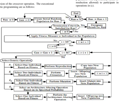
Figure 2 is a flowchart of genetic programming showing the genetic operations of crossover, reproduction, and mutation as well as the architecture-altering operations. This flowchart shows a two-
offspring version of the crossover operation. The executional steps of genetic programming are as follows:
1. Randomly create an initial population (generation 0) of individual computer programs composed of the available functions and terminals.
2. Iteratively perform the following sub-steps (called a generation) on the population until the termination criterion is satisfied:
a. Execute each program in the population and ascertain its fitness (explicitly or implicitly) using the problem’s fitness measure.
b. Select one or two individual program(s) from the population with a probability based on fitness (with reselection allowed) to participate in the genetic operations in (c).
Figure 3.1: Flowchart of the Genetic Program
c. Create new individual program(s) for the population by applying the following genetic operations with specified probabilities:
i. Reproduction: Copy the selected individual program to the new population.
ii. Crossover: Create new offspring program(s) for the new population by recombining randomly chosen parts from two selected programs.
iii. Mutation: Create one new offspring program for the new population by randomly mutating a randomly chosen part of one selected program.
iv. Architecture-altering operations: Choose an architecture-altering operation from the available repertoire of such operations and create one new offspring program for the new population by applying the chosen architecture-altering operation to one selected program.
After the termination criterion is satisfied, the single best program in the population produced during the run (the best-so-far individual) is harvested and designated as the result of the run. If the run is successful, the result may be a solution (or approximate solution) to the problem.
3.3
Model Simulation Process and Environment
Following the identification of the algorithms that were needed for the formulation of the predictive model for the risk of kidney disease, the simulation of the predictive model was performed using the data collected which consisted of individuals records containing information about the risk factors and their respective risk of kidney diseases from a hospital in south-western Nigeria. The WEKA software – a suite of machine learning algorithms was used as the simulation environment for the development of the predictive model. [image:6.595.100.496.201.543.2]process of training and testing predictive model according to literature is a very difficult experience especially with the various available validation procedures. For this classification problem, it was natural to measure a classifier’s performance in terms of the error rate. The classifier predicted the class of each instance – the pregnant women’s record containing values for each risk of kidney disease: if it is correct, that is counted as a success; if not, it is an error. The error rate being the proportion of errors made over a whole set of instances, and thus measured the overall performance of the classifier. The error rate on the training data set was not likely to be a good indicator of future performance; because the classifiers were been learned from the very same training data.
In order to predict the performance of a classifier on new data, there was the need to assess the error rate of the predictive model on a dataset that played no part in the formation of the classifier. This independent dataset was called the test dataset – which was a representative sample of the underlying problem as was the training data. It was important that the test dataset was not used in any way to create the classifier since the machine learning classifiers involve two stages: one to come up with a basic structure of the predictive model and the second to optimize parameters involved in that structure.
The process of leaving a part of a whole dataset as testing data while the rest is used for training the model is called the holdout method. The challenge here is the need to be able to find a good classifier by using as much of the whole historical data as possible for training; to obtain a good error estimate and use as
much as possible for model testing. It is a common trend to holdout one-third of the whole historical dataset for testing and the remaining two-thirds for training.
For this study the cross-validation procedure was employed, which involved dividing the whole datasets into a number of folds (or partitions) of the data. Each partition was selected for testing with the remaining k – 1 partitions used for training; the next partition was used for testing with the remaining k – 1 partitions (including the first partition used or testing) used for training until all k partitions had been selected for testing. The error rate recorded from each process was added up with the mean the mean error rate recorded. The process used in this study was the stratified 10-fold cross validation method which involves splitting the whole dataset into ten partitions.
3.4
Performance Evaluation of Model
Validation Process
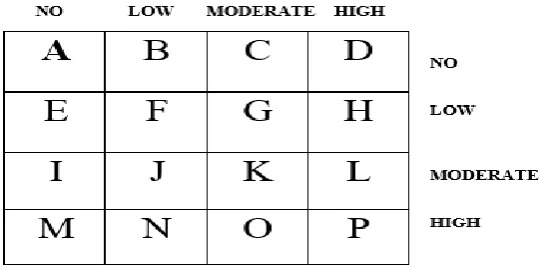
During the course of evaluating the predictive model, a number of metrics were used to quantify the model’s performance. In order to determine these metrics, four parameters must be identified from the results of predictions made by the classifier during model testing. These are: true positive (TP), true negative (TN), false positive (FP) and false negative (FP). True positives/negatives are correct classifications while false positives/negatives are incorrect classifications/misclassifications. These results are presented on confusion matrix – for this study the confusion matrix is a 4 x 4 owing to the three labels for the output class – risk of kidney diseases, namely: no, low, moderate and high risk.
[image:7.595.171.445.433.568.2]Figure 3.2 shows the diagram of the confusion matrix that was used for evaluating the performance of the decision trees algorithms developed in this study. Each cell in the 4 x 4 matrix represents the correct/incorrect classification depending on the cell referenced.
Figure 3.2: Confusion matrix diagram for performance evaluation
The values of the cells are in turn used to estimate the performance metrics. The sum of the values of the cells across provides the number of actual cases in the training dataset while the sum of the columns provide the number of predicted cases in the training dataset. The cells located on the diagonal are the correct classifications (true positives/negatives) while other cells are the misclassifications/incorrect classifications (false positives/negatives). The performance metrics are thus defined as follows:
Sensitivity/True positive rate/Recall: is the proportion of actual cases that were correctly predicted.
False Positive rate/False alarm: is the proportion of actual cases that were incorrectly predicted.
and
.
Precision: is the proportion of the predicted cases that were correctly predicted.
Accuracy: is the total number of correct classifications (positive and negative)
4.
RESULTS AND DISCUSSION OF THE
MODEL
4.1
Results and Discussion of Data
Identification and Collection
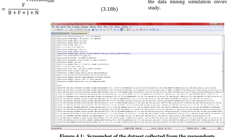
[image:8.595.60.270.68.269.2]For this study, data was collected from 45 patients using the questionnaires constructed for this study among which; the risk of kidney disease was identified. Figure 4.1 shows a screenshot of the data collected from the 45 respondents selected for this study. The data was stored in the attribute relation file format (.arff) which is the acceptable format for the data mining simulation environment selected for this study.
Figure 4.1: Screenshot of the dataset collected from the respondents
The format required the identification of three (3) parts of the dataset, namely:
a. The relation section: was used to identify the name of the file identified which in this case is kidney-stones-data for the data containing all 30 patients selected for training and testing the model after. The relations tag is identified using the name @relation before the relation name;
b. The attribute section: was used to identify the fields/attributes (risk factors) identified as the input variables for the risk of kidney disease where the last attributes describes the risk of hypertension. There are 33 attributes identified in the file with the first 32 identifying the input variables (risk factors of the risk of kidney disease) while the last variable is the risk of kidney disease. Each attribute has its own respective label which shows the possible values that can be stated by each
attribute defined in the dataset. The attribute tag for each attribute is identified using the name @attribute before each attribute name; and
c. The data section: was used to identify the dataset values for each respondents collected in the same order as the attributes were listed. Each respondent’s record of data is represented as the set of values on each line with the risk of kidney disease shown on the last portion of each line. The data containing the values of the attributes for each respondent is listed on the line following the name tag identified as @data.
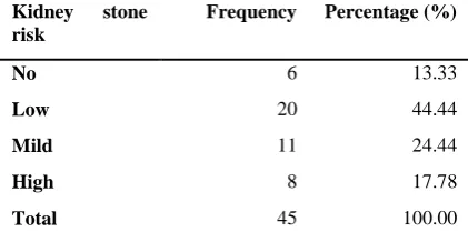
[image:8.595.66.449.346.577.2]Table 4.1: Distribution of kidney disease risk among historical dataset
Kidney stone risk
Frequency Percentage (%)
No 6 13.33
Low 20 44.44
Mild 11 24.44
High 8 17.78
Total 45 100.00
The table shows that out of the 45 patients considered; 6 (13.3%) had no risk of kidney disease, 20 (44.4%) had low risk of kidney disease, 11 (24.4%) had moderate risk of kidney disease while 8 (17.8%) had high risk of kidney disease. It was observed that the highest case presented was for respondents with low risk of kidney disease while the least case was presented for respondents with no risk of kidney disease. Tables 4.2 and 4.3 gives a description of the nominal data collected from all 45 respondents selected for the study; they show the distribution of the demographic variables and risk factors of kidney diseases respectively defined for the dataset collected from the respondents.
Based on the information presented in Table 4.2, the frequency distribution of the responses of the demographic information of the patients is presented. Regarding the age of the patients selected, majority of the patients selected for this study were within the age group of 19 to 35 years of age and 11 to 18
years of age; regarding the education of the respondents, majority attended polytechnic/university representing about 50% of the respondents followed by those who attended secondary schools representing about 22% of the respondents selected for the study.
[image:9.595.103.493.424.763.2]The results further showed that majority of the respondents were single which was represented by 60% of the respondents; regarding the ethnicity of the patients selected, majority were Yoruba represented by about 90% of the patients while about 70% of the patients were observed to be Christian. The results also further showed that about 70% of the patients had a normal body mass index (BMI) showing indications of good nutrition but about 15% of the patients were observed to have a BMI value of underweight showing indications of a very poor diet. The description of the risk factors is presented in Table 4.3below
Table 4.2: Description of the demographic variables of the patients collected
Demographic Information Labels Frequency (%)
Age (years) 11-18
19-35
above 35
14 (31.11)
19 (42.22)
12 (26.67)
Education Secondary
NCE
Polytechnic
University
Missing
10 (22.22)
8 (17.78)
12 (26.67)
12 (26.67)
3 (6.67)
Occupation Civil Servant
Student
Trader
Artisan
Teacher
9 (20.00)
17 (37.78)
7 (15.56)
3 (6.67)
9 (20.00)
Marital Status Single
Married
27 (60.00)
18 (40.00)
Ethnicity Yoruba
Hausa
39 (86.67)
Ibo
Igala
2 (4.44)
1 (2.22)
Religion Islam
Christianity
Traditional
Missing
10 (22.22)
33 (73.33)
1 (2.22)
1 (2.22)
BMI Class Underweight
Normal
Overweight
Class I obese
Class II obese
Class III obese
6 (13.33)
31 (68.89)
4 (8.89)
3 (6.67)
0 (0.00)
[image:10.595.103.492.312.763.2]1 (2.22)
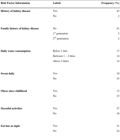
Table 4.3: Description of the risk factor information of the patients collected
Risk Factor Information Labels Frequency (%)
History of kidney disease Yes
No
43
2
Family history of kidney disease No
1st generation
2nd generation
41
2
2
Daily water consumption Below 1 litre
Between 1 – 2 litres
Above 2 litres
17
14
14
Sweat daily Yes
No
10
35
Obese since childhood Yes
No
12
33
Stressful activities Yes
No
27
18
Eat late at night Yes
No
21
Vegetarian Yes
No
27
17
Take coffee Yes
No
32
13
Coffee cups consumed Nil
1 daily
Above 1 daily
1 weekly
Above 1 weekly
13
12
5
11
4
Consume soft-drinks Yes
No
37
8
Amount of salt in diet Below 1 tablespoon
Above 1 tablespoon
41
4
Consumption of processed foods Daily
Weekly
Missing
24
20
1
Smoke Yes
No
4
41
Frequency of smoking Nil
1 pack daily
1 pack weekly
1 pack monthly
40
2
2
1
Consumption of soya milk Yes
No
29
16
Frequency of soya milk consumption Nil
Daily
Weekly
Monthly
16
7
14
Consumption of alcohol Yes
No
8
37
Alcohol frequency Nil
Daily
Weekly
Monthly
39
2
3
1
Family history of diabetes No
1st generation
2nd generation
44
0
1
Family history of hypertension No
1st generation
2nd generation
40
2
3
Family history of Urinary Tract Infection (UTI)
No
1st generation
2nd generation
42
0
3
4.2
Results of Model Formulation and
Simulation
Following the identification of the risk factors that are associated with kidney stones risk, the next phase is model formulation using the aforementioned decision trees algorithms available in the WEKA software. The 10-fold cross validation technique was used in evaluating the performance of the developed predictive model for kidney stones risk using the historical dataset used for training the model.
From the dataset collected from the respondents, the training data was used for the formulation of the predictive model needed for the prediction of the risk of kidney stones. The J4.8 decision trees algorithm was used to implement the C4.5 decision trees algorithm for the formulation of the predictive model using the simulation environment. The results of the model formulation using C4.5 decision trees was used to identify some relevant variables indicative of kidney stones disease. These variables were used to formulate the predictive model using the genetic programming and the multi-layer perceptron.
4.2.1
Results of the Model Formulation and
Identification of Relevant Variables
The results of the formulation of the predictive model for the risk of kidney stones using the C4.5 decision trees algorithm showed that six (6) variables were the most important risk factors of kidney stones and were used by the algorithm to develop the tree that was used in formulating the predictive model for risk of Kidney stone using the C4.5 decision trees
algorithm. The variables identified in the order of their importance were:
a. Obese since childhood;
b. Family history of hypertension;
c. Coffee consumption;
d. BMI class;
e. Eat late at night; and
f. Sweat daily.
Based on the six (6) variables identified by the C4.5 decision trees algorithm, the predictive model for the risk of kidney stones was formulated based on the results of the simulation using the J48 decision trees algorithm on the WEKA simulation environment. Figure 4.2 shows the decision trees that was formulated based on the six (6) variables that was proposed by the algorithm. The tree was used to deduce the set of rules that were proposed for determining the risk of kidney stones based on the values of the variables identified by the algorithm. In all, there were 13 rules extracted by the C4.5 decision trees algorithm. The rules extracted from the tree are as follows:
i. If (obese from childhood=no) and (family history of hypertension=no) and (take coffee=yes) and BMI class=overweight) then kidney risk=No
iii. If (obese from childhood=no) and (family history of hypertension=no) and (take coffee=yes) and BMI class=normal) and (eat late=yes) and (sweat daily=yes) then kidney risk=Moderate
iv. If (obese from childhood=no) and (family history of hypertension=no) and (take coffee=yes) and BMI
class=normal) and (eat late=no) then kidney risk=Low
[image:13.595.141.456.154.337.2]v. If (obese from childhood=no) and (family history of hypertension=no) and (take coffee=yes) and BMI class=class I obese) then kidney risk=Low
Figure 4.2: Decision Tree formulated using C4.5 for Risk of Kidney stones
vi. If (obese from childhood=no) and (family history of hypertension=no) and (take coffee=yes) and BMI class=class II obese) then kidney risk=Low
vii. If (obese from childhood=no) and (family history of hypertension=no) and (take coffee=yes) and BMI class=class III obese) then kidney risk=High
viii. If (obese from childhood=no) and (family history of hypertension=no) and (take coffee=yes) and BMI class=overweight) then kidney risk=Low
ix. If (obese from childhood=no) and (family history of hypertension=no) and (take coffee=no) and (eat late=yes) then kidney risk=Low
x. If (obese from childhood=no) and (family history of hypertension=no) and (take coffee=no) and (eat late=no) then kidney risk=No
xi. If (obese from childhood=no) and (family history of hypertension=first) then kidney risk=Low
xii. If (obese from childhood=no) and (family history of hypertension=second) then kidney risk=Moderate
xiii. If (obese from childhood=yes) then kidney risk=High
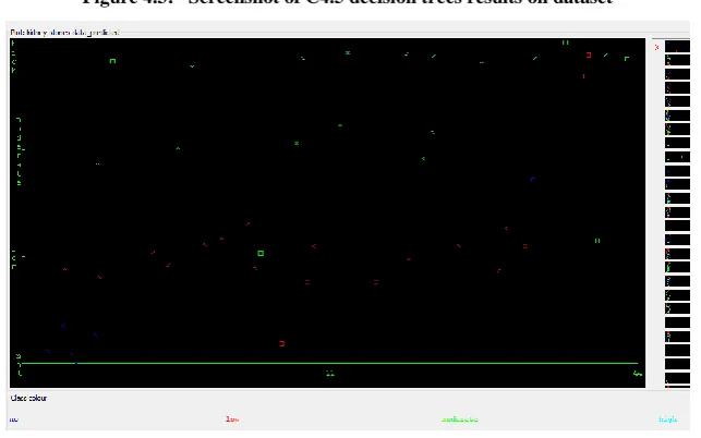
Figure 4.3: Screenshot of C4.5 decision trees results on dataset
Figure 4.4: Screenshot of correct and incorrect classifications made by C4.5
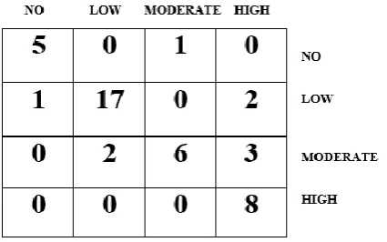
The results presented in Figure 4.4 was used to evaluate the performance of the C4.5 decision trees algorithm and thus, the confusion matrix determined. Figure 4.5 shows the confusion matrix that was used to interpret the results of the true positive and negative alongside the false positive and negatives of the validation results. The confusion matrix shown in Figure 4.5 was used to evaluate the performance of the predictive model for risk of kidney stones. From the confusion matrix shown in Figure 4.5, the following sections present the results of the model’s performance. Out of the 6 actual no cases, 5 were correctly classified as no while 1 was misclassified as moderate risk, out of the 20 actual low cases, there were 17 correct classifications with 1 misclassified as no risk and 2 misclassified as high risk; out of the 11 moderate risk cases, there were 6 correct classifications with 2 misclassified as no risk and 3 misclassified as high risk while out of the 8 high cases, all were correctly classified. Therefore, there were 36
correct classifications out of the 45 records considered for the model development owing for an accuracy of 80%.
4.2.2
Results of Model Formulation Using the
Genetic Programming
[image:14.595.138.460.301.502.2]Figure 4.5: Confusion matrix of performance evaluation using C4.5
of kidney stones. The genetic programming algorithm was used for the formulation of the predictive model using the simulation environment.
Following the simulation of the predictive model for risk of kidney stones using the genetic programming algorithm, the evaluation of the performance of the model following validation using the 10-fold cross validation method was recorded using all the initially variables and using the variables selected by the C4.5 decision trees algorithm. Figure 4.6 shows the screenshot of the results of the predictions made by the genetic programming algorithm for the 45 instances of data collected from the patients considered for this study containing the initial 33 variables (Figure 4.6 left) and the final 6 variables (Figure 4.6 right). The Figures in Figure 4.6 shows the correct
and incorrect classifications made by the algorithm while Figure 4.7 shows the graphical plot of the predictions made by the genetic programming algorithm on the dataset.
In Figure 4.7, each class of kidney stones is represented using a specific colour and each correct classification is represented with a star while each misclassification is represented as a square. Figure 4.7-top shows the graphical plot of the results of the genetic programming algorithm using the initial 33 variables while Figure 4.7-bottom shows the graphical plot of the results of the genetic programming algorithm using the 6 variables selected by the C4.5 decision trees algorithm. The results presented in Figure 4.7 was used to evaluate the performance of the genetic programming algorithm and thus,
the confusion matrix determined.
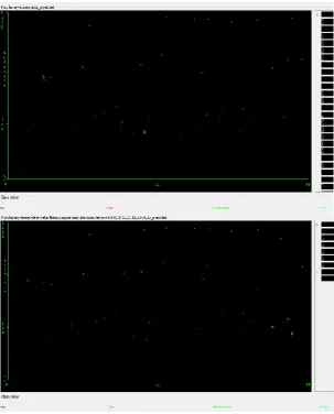
[image:15.595.106.496.427.644.2]
Figure 4.7: Screenshot of correct and incorrect classifications made by genetic programming using initial 33 variables (top) and 6 variables selected by C4.5 decision trees (bottom)
Figure 4.8 shows the confusion matrix that was used to interpret the results of the true positive and negative alongside the false positive and negatives of the validation results. The confusion matrix shown in Figure 4.8 was used to evaluate the performance of the predictive model for risk of kidney stone disease. Figure 4.8-left shows the confusion matrix for the results of the genetic programming algorithm using the initial 33 variables while Figure 4.8-right shows the results of the genetic programming algorithm using the 6 variables selected by the C4.5 decision trees algorithm. From the confusion matrix shown in Figure 4.8, the following sections present the results of the model’s performance.
Based on the confusion matrix shown in Figure 4.8-left, out of the 6 actual no risk, 5 were correctly classified while 1 was misclassified as low risk, out of the 20 actual low cases, there were 19 correct classifications with 1 misclassified as moderate risk; out of the 11 moderate risk cases, there were 9 correct
classifications with 2 misclassified as low risk and out of the 8 high cases, there were 7 correct classifications with 1 misclassified as low risk. Therefore, there were 40 correct classifications out of the 45 records considered for the model development owing for an accuracy of 88.9%.
Based on the confusion matrix shown in Figure 4.8-right, out of the 6 actual no risk, 5 were correctly classified while 1 was misclassified as moderate risk, out of the 20 actual low cases, there were 18 correct classifications with 1 misclassified as moderate risk and 1 misclassified as high; out of the 11 moderate risk cases, there were 9 correct classifications with 2 misclassified as low risk and out of the 8 high cases, there were 7 correct classifications with 1 misclassified as low risk. Therefore, there were 40 correct classifications out of the 45 records considered for the model development owing for an
Figure 4.8: Confusion matrix of performance evaluation of genetic programming using initial 33 variables (left) and variables selected by C4.5 decision trees algorithm (right)
The results of the performance of the genetic programming algorithm shows that the performance of the genetic programming algorithm was not improved by the variables identified by the C4.5 decision trees algorithm rather the performance was better using the initial 33 variables than using the selected 6 variables by the C4.5 decision trees algorithm. This may be partly due to the ability of the genetic programming algorithm to select the variables which optimize its performance using the laws of natural selection.
4.2.3
Results of Model Formulation Using
Multi-Layer Perceptro
nFollowing the formulation of the predictive model for the risk of kidney stones, the next phase was model formulation using the multi-layer perceptron available in the WEKA software. The 10-fold cross validation technique was used in evaluating the performance of the developed predictive model for kidney stones risk using the historical dataset used for training the model. This process was performed and compared with the performance of the predictive model developed using the variables selected by the C4.5 decision trees algorithm for the most effective. From the dataset collected from the respondents, the training data was used for the formulation of the predictive model needed for the prediction of the risk of kidney stones. The multi-layer perceptron was used for the formulation of the predictive model using the simulation environment.
Following the simulation of the predictive model for risk of kidney stones using the multi-layer perceptron, the evaluation of the performance of the model following validation using the 10-fold cross validation method was recorded using all the initially variables and using the variables selected by the C4.5
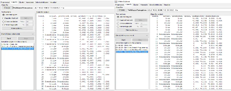
decision trees algorithm. Figure 4.9 shows the screenshot of the results of the predictions made by the multi-layer perceptron for the 45 instances of data collected from the patients considered for this study containing the initial 33 variables (Figure 4.9 left) and the final 6 variables (Figure 4.9 right). The Figures in Figure 4.9 shows the correct and incorrect classifications made by the algorithm while Figure 4.10 shows the graphical plot of the predictions made by the multi-layer perceptron on the dataset.
In Figure 4.10, each class of kidney stones is represented using a specific colour and each correct classification is represented with a star while each misclassification is represented as a square. Figure 4.10-top shows the graphical plot of the results of the multi-layer perceptron using the initial 33 variables while Figure 4.10-bottom shows the graphical plot of the results of the multi-layer perceptron using the 6 variables selected by the C4.5 decision trees algorithm. The results presented in Figure 4.10 was used to evaluate the performance of the multi-layer perceptron and thus, the confusion matrix determined.
Figure 4.11 shows the confusion matrix that was used to interpret the results of the true positive and negative alongside the false positive and negatives of the validation results. The confusion matrix shown in Figure 4.11 was used to evaluate the performance of the predictive model for risk of kidney stone disease. Figure 4.11-left shows the confusion matrix for the results of the multi-layer perceptron using the initial 33 variables while Figure 4.11-right shows the results of the multi-layer perceptron using the 6 variables selected by the C4.5 decision trees algorithm. From the confusion matrix shown in Figure 4.11, the following sections present the results of the
model’s performance.
[image:17.595.100.496.566.722.2]Figure 4.10: Screenshot of correct and incorrect classifications made by multi-layer perceptron using initial 33 variables (top) and 6 variables selected by C4.5 decision trees (bottom)
Figure 4.11: Confusion matrix of performance evaluation of multi-layer perceptron using initial 33 variables (left) and variables selected by C4.5 decision trees algorithm (right)
Based on the confusion matrix shown in Figure 4.11-left, out of the 6 actual no risk, all were correctly classified, out of the 20 actual low cases, all were correctly classified, out of the 11 moderate risk cases, all were correctly classified and out of the 8 high cases, all were correctly classified. Therefore, all 45 records were correctly classified for the model development owing for an accuracy of 100%.
Based on the confusion matrix shown in Figure 4.11-right, out of the 6 actual no risk, 5 were correctly classified while 1 was misclassified as moderate risk, out of the 20 actual low cases, there were 18 correct classifications with 2 misclassified as high risk, out of the 11 moderate risk cases, there were 9 correct classifications with 1 misclassified as no risk while 1 was misclassified as high risk and out of the 8 high cases, all were correctly classified. Therefore, there were 40 correct
classifications out of the 45 records considered for the model development owing for an accuracy of 86.7%.
The results of the performance of the multi-layer perceptron shows that the performance of the multi-layer perceptron was not improved by the variables identified by the C4.5 decision trees algorithm rather the performance was better using the initial 33 variables than using the selected 6 variables by the C4.5 decision trees algorithm. The multi-layer perceptron was able to correctly classify all instances containing information about the risk factors of kidney stones using all 33 initial variables identified. Therefore, by reducing the variable from 33 to 6 the multi-layer perceptron had lost important information needed for the formulation of the predictive model for kidney stones.
[image:18.595.146.461.458.570.2]4.3
Discussion of Results
The result of the performance evaluation of the machine learning algorithms are presented in Table 4.3 which presents the average values of each performance evaluation metrics considered for this study. For the C4.5 decision trees algorithm based on the results presented in the confusion matrix presented in Figure 4.5. The results showed that the TP rate which gave a description of the proportion of actual cases that was correctly predicted was 0.807 which implied that 80% of the actual cases were correctly predicted; the FP rate which gave a description of the proportion of actual cases misclassified was 0.068 which implied that 7% of actual cases were misclassified while the precision which gave a description of the proportion of predictions that were correctly classified was 0.800 which implied that 80% of the predictions made by the classifier were correct.
For the genetic programming algorithm based on the results presented in the confusion matrix presented in Figure 4.8. The results of using the initially identified 33 variables showed that the TP rate which gave a description of the proportion of actual cases that was correctly predicted was 0.869 which implied that 87% of the actual cases were correctly predicted; the FP rate which gave a description of the proportion of actual cases misclassified was 0.047 which implied that 5% of actual cases were misclassified while the precision which gave a description of the proportion of predictions that were correctly classified was 0.931 which implied that 93% of the predictions made by the classifier were correct.
The results of using the 6 variables identified by the C4.5 decision trees algorithm showed that the TP rate which gave a description of the proportion of actual cases that was correctly predicted was 0.857 which implied that 86% of the actual cases were correctly predicted; the FP rate which gave a description of the proportion of actual cases misclassified was 0.052 which implied that 5% of actual cases were misclassified while the precision which gave a description of the proportion of predictions that were correctly classified was 0.888 which implied that 89% of the predictions made by the classifier were correct.
For the multi-layer perceptron algorithm based on the results presented in the confusion matrix presented in f 4.11. The results of using the initially identified 33 variables showed that the TP rate which gave a description of the proportion of actual cases that was correctly predicted was 1 which implied that all of the actual cases were correctly predicted; the FP rate which gave a description of the proportion of actual cases misclassified was 0 which implied that none of actual cases were misclassified while the precision which gave a description of the proportion of predictions that were correctly classified was 1 which implied that all of the predictions made by the classifier were correct.
The results of using the 6 variables identified by the C4.5 decision trees algorithm showed that the TP rate which gave a description of the proportion of actual cases that was correctly predicted was 0.888 which implied that 89% of the actual cases were correctly predicted; the FP rate which gave a description of the proportion of actual cases misclassified was 0.034 which implied that 3% of actual cases were misclassified while the precision which gave a description of the proportion of predictions that were correctly classified was 0.865 which implied that 87% of the predictions made by the classifier were correct.
[image:19.595.64.537.510.703.2]In general, the multi-layer perceptron and the genetic programming algorithms were able to predict the risk of kidney stones better than the C4.5 decision trees algorithm. The results further showed that the use of the variables identified by the decision trees algorithm to formulate the predictive model did not improve the performance of the multi-layer perceptron and the genetic programming algorithm used for this study. Overall, the multi-layer perceptron was able to accurately classify all cases of kidney stones with a value of 100% showing that it had the capacity to identify the complex patterns that existed within the dataset than the genetic programming and the C4.5 decision trees algorithm. The variables identified by the C4.5 decision trees algorithm can also be given very close attention and observed in order to better understand the risk of kidney stones in patients monitored by the endocrinologists.
Table 4.3: Summary of the results of performance evaluation for the machine learning algorithms selected
Machine Learning Algorithm Used
Variables Applied
PERFORMANCE EVALUATION METRICS
Correct Classificati
on (out of 45)
Accuracy (%)
TP rate (recall/sensitiv
ity)
FP rate (false positive)
Precision
C4.5 Decision Trees Algorithm
33 36 80.0 0.807 0.068 0.800
Genetic Programming Algorithm
33 40 88.9 0.869 0.047 0.931
6 39 86.7 0.857 0.052 0.888
Multi-Layer Perceptron Algorithm
33 45 100.0 1.000 0.000 1.000
6 40 88.9 0.888 0.034 0.865
5.
CONCLUSION
This paper focused on the development of a prediction model using identified risk factors in order to classify the risk of kidney stones in selected respondents for this study. Historical dataset